F. Random Errors
1. Concepts
Once mistakes have been removed and systematic errors compensated, the only errors left are random. They tend to be small and as likely to be positive as negative. If enough measurements are made (under the same conditions, with the same equipment) they would cancel out.
Random errors behave according to laws of probability. An example is flipping a coin. Disregarding the apparent weight differential between the faces, there’s a 50-50 chance heads will come up. It’s possible that if we flip it twice it will come up heads both times. Flipping it three times we could get none, one, two, or three heads. The more we flip it, the more likely we’ll approach 50-50 on heads coming up. Theoretically, if you flip the coin an infinite number of times, keeping everything else the same, half the time it will come up heads. Don’t believe me? Give it a try, I’ll wait.
Anyway, the more times something is measured, the better the result. Unfortunately we don't have the luxury of time to make an infinite number of measurements (nor a client willing to pay for it). How many times to measure depends on overall accuracy needed and equipment used.
Statistics are used to analyze or predict random error behavior. Statistics allows precision determination and accuracy prediction for a measurement set. They can also help plan how measurements should be made to meet an expected accuracy level.
Random error behavior and analysis can get complicated very quickly particularly when mixed-quality measurements are combined in a network. Our objective is to understand basic terminology and analysis tools. If you are interested in more advanced aspects of random error behavior, there are a few very good textbooks on the subject.
2. Statistics
How many measurements must be made to be statistically significant? Good question, and not an easy one to answer. We know that at least three measurements should be made in order to trap mistakes, but three is pretty light. Once we introduce some analysis equations, we'll be able to make some predictions. For now, we'll use a small measurement set to explain some terms and statistical analyses.
Our sample measurement set is: 45.66 45.66 45.68 45.65
a. Discrepancy
The difference between any two measurements of the same quantity.
Example: the discrepancy between the highest and lowest measurements is 0.03
b. Most Probable Value (MPV)
This is a fancy way of saving average or mean. In simplest form, it's the measurement sum divided by the number of measurements.
 |
Equation F-1 |
|
MPV: most probable vlaue |
|
Example: MPV = (45.66+45.66+45.68+45.65)/4 = 45.662
In analyses where mixed-quality measurements are combined the MPV might be called a “weighted average.” This takes into account quality variations giving higher consideration to better quality measurements. For our purposes, measurements will be made using consistent instrumentation and procedures so we will use an unweighted average (also called a unit weight average).
c. Residual (v)
The difference between a measurement and the MPV. This is like a discrepancy except it’s always compared against the MPV.
Example: Residual of the first measurement is 45.66-45.662 = -0.002
It doesn't really matter if the MPV is subtracted from the measurement or vice versa since we will ultimately square each so the mathematical sign goes away. Just be consistent: (measurement-MPV) or (MPV - measurement).
d. Normal Distribution Curve
Computing all the residuals and plotting their frequency results in a bell-shaped curve, Figure F-1. The curve is symmetric with smaller residuals more frequent and grouped closer to the MPV. The curve is asymptotic: it approaches the x-axis but never touches it.
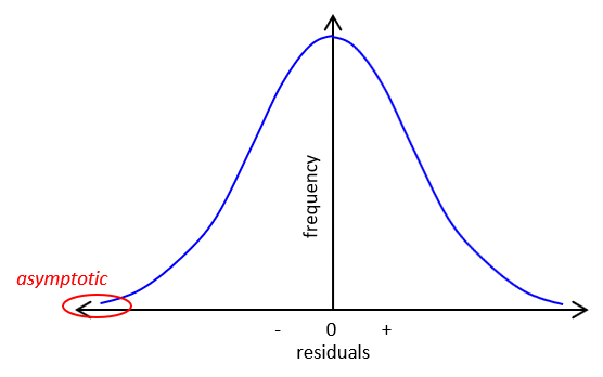 |
| Figure F-1 Normal Distribution Curve |
Of course with only four measurements in this example, ours would be a pretty sorry looking bell. Just like flipping the coin, as you approach an infinite number of measurements your graph becomes a smooth curve.
e. Standard Deviation
On both sides of the curve is an inflection point: where the curve changes from convex to concave. These occur at ±σ along the x-axis, Figure F-2.
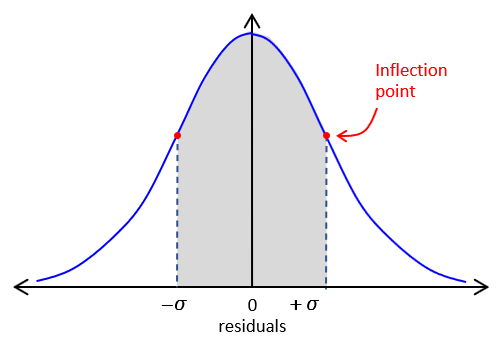 |
| Figure F-2 Standard Deviation |
To compute the standard deviation:
 |
Equation G-2 | |
| σ: standard deviation v: residual n: number of measurements |
||
You’ll also see another form of the equation:
 |
Equation F-3 |
What's the difference? This is a little over-simplified, but basically:
Equation F-2 is used for a subset of all the data (sample set)
Equation F-3 is used with an entire data set (entire population)
Equation F-3 is referred to as the Standard Error. It's used when an entire data set us available for measurement. Standard deviation is used when it's not practical to analyze all the data.
Example:
To determine the compressive strength of concrete that will be used to build a structure, test cylinders of the fresh concrete are poured and then destructively tested at 7, 30, and 365 days. To determine the concrete's average strength and its standard error, all the concrete would be tested (entire population) leaving nothing with which to build the structure. That is neither practical nor economically feasible. Instead, random samples are taken from batch mixes and tested. From this sample subset we determine the average strength and its standard deviation.
In surveying, we attempt to determine an unknown quantity by measurement. The entire population can only be attained with an infinite number of measurements. We are limited to a finite number of measurements - we collect a sample of the entire population. So to analyze our measurements, we use the standard deviation from Equation G-2. The larger the sample set, the better the statistical analysis.
Adding to the confusion, some texts use σ for standard deviation and S for standard error while others use S for standard deviation and σ for standard error. Whatever it's called, remember: in measurement science we work with a sample set so always use (n-1) in the denominator.
Note that as n increases, the difference between Equations F-2 and F-3 decreases. When n hits infinity, division by either infinity or (infinity-1) makes little difference.
Anyway, back to standard deviation, Equation F-2...
This area bounded by ±σ and the curve is ~68.3% of the total area under the entire normal distribution curve. What that means is ~68% of our measurements fall within ±σ of the MPV.
Standard deviation is an indicator of the measurement set's precision: the smaller the standard deviation, the smaller the data spread, the better the precision. Figure F-3 demonstrates this for two different measurement sets.
 |
| Figure F-3 Standard Deviation and Precision |
f. Confidence Interval (CI)
A confidence interval is the degree of certainty that a value falls within a specific range. The standard deviation represents a 68.3% confidence interval: continuing measurements under similar conditions using similar equipment and procedures, we’re 68.3% confident that our results will fall within ±σ of our MPV.
Other common CIs are 90% and 95%:
The 90% CI covers 90% of the area under the normal distribution curve. It’s roughly equal to 1.65 times the standard deviation. Measurements are expected to fall between ±1.65σ of the MPV 90% of the time.
The 95% CI, which includes 95% of the area under the curve, is roughly equal to 1.96 times the standard deviation. Being so close to 2 it is sometimes referred to as the 2 sigma (2σ) confidence. Measurements are expected to fall between ±2σ of the MPV 95% of the time.
Hey, what about 100% confidence? After all, we spent all this money on expensive equipment so we should be able to state 100% confidence, right? Well, you can. Since the normal distribution curve is asymptotic you can state with 100% confidence that your measurement will fall within ±infinity of the MPV.
g. Standard Error Of the Mean
This the expected error in the MPV. Since we don’t know the exact error present, this is only an indicator. It’s computed from:
 |
Equation F-4 | |
| EMPV: Error off the mean σ: standard deviation n: number of measurements |
||
Note that it’s a function of the standard deviation and number of measurements. Theoretically, as the number of measurements increases, EMPV decreases: less error with more measurements since the random errors get more chances to cancel.
Standard error of the mean is an indicator of accuracy.
3. Example Computations
a. Measurement Set
Let's compute the statistics of our measurement set: 45.66 45.66 45.68 45.65
(Keep in mind that this is an absurdly small measurement set hardly worthy of statistical analysis. We're using it only to demonstrate the random error analysis process).
| Step (1) | Step (2) | Step (3) | |
| num | value | v = meas-MPV | v2 |
| 1 | 45.66 | 45.66-45.662 = -0.002 | 0.000004 |
| 2 | 45.66 | 45.66-45.662 = -0.002 | 0.000004 |
| 3 | 45.68 | 45.68-45.662 = +0.018 | 0.000324 |
| 4 | 46.65 | 45.65-45.662 = -0.012 | 0.000144 |
| sums | 182.65 | 0.000476 |
(1) Compute MPV, Equation F-1
According to the rules of significant figures, the measurement sum has 5 sig fig.
In addition to isolating errors, repeating measurements can also increase accuracy. In this case, we’ve gone from 0.01 units to 0.001 units. Of course, the more measurements made, the stronger that additional accuracy. Four measurements, as in our example, are not really enough for a true statistical picture.
(2) Compute the residuals

Since this represents an intermediate computation, carry an additional digit. Residuals have the same units as the measurements.
(3) Square and sum the residuals
Keeping in mind the addition rule for significant figures, the measurement sum has 3 sig fig.
By the way, the term least squares comes from the fact the MPV is the number which results in the smallest (or least) sum of the squares of the residuals. Any other number will result in a larger sum.
(4) Compute the standard deviation, Equation F-2
The standard deviation has the same units as the measurements.
(5) Compute the Error of the MPV, Equation F-4
The error of the MPV has the same units as the measurements.
(6) Results
From (1), the MPV is good to 0.001
We should express the standard deviation and error of the mean to the same resolution level.
MPV = 45.662 ±0.013; EMPV = ±0.006
So what’s all this mean? Based on our measurements:
- The most probable value of the measured quantity is 45.662;
- 68% of our measurements fall within ±0.013 of the MPV;
- The error in the MPV is expected to be ±0.006.
b. Example with Angles
One of the problems working with angles is the tendency to carry insufficient digits when converting from deg-min-sec to decimal degrees. For some reason, three decimal places seems to be the norm but this can cause substantial rounding error computing measurement statistics.
To demonstrate this, lets look at a simple example consisting of 4 angles: 168°42'30", 168°42'10", 168°42'15", and 168°42'25".
(1) Convert to and carry three decimal places.
| Angle | Decimal Deg | v; deg | v2; deg2 |
| 168°42'30" | 168.708 | +0.002 | 0.000004 |
| 168°42'10" | 168.703 | -0.003 | 0.000009 |
| 168°42'15" | 168.704 | -0.002 | 0.000004 |
| 168°42'25" | 168.707 | +0.001 | 0.000001 |
| sums: | 674.822 | 0.000018 |

The computations aren't too onerous (a byproduct of using only three decimal places). However, once the angles are converted to decimal degrees, it's difficult to interpret magnitudes of subsequent calculations. Residuals are in decimal degrees; what are those in terms of the original mixed units? It's hard to judge if the residuals (and MPV, SD, EMPV) make sense for the measurement set.
(2) Convert to and carry seven decimal places
| Angle | Decimal Deg | v; deg | v2; deg2 |
| 168°42'30" | 168.7083333 | +0.0027777 | 0.0000077156 |
| 168°42'10" | 168.7027778 | -0.0027778 | 0.0000077162 |
| 168°42'15" | 168.7041667 | -0.0013889 | 0.0000019290 |
| 168°42'25" | 168.7069444 | +0.0013888 | 0.0000019288 |
| sums: | 674.8222222 | 0.0000192896 |

While the process is the same as the first, two things are readily apparent
- There are a lot more numbers to write down and uses in calculations
- The additional four decimal places have a significant impact the MPV, SD, and EMPV values.
Conclusion? Carrying only three decimal places results in substantial intermediate rounding. As we learned in the Significant Figures chapter, carrying more digits than needed and rounding at the end means less biased results.
But seven decimal places are sooooo many to carry. Would six be enough? Five? Four? We discussed how to convert angles to decimal degrees to the correct number of sig fig in the Significant Figures chapter. Although we could determine how many decimal places are needed, we still have the same issue as before: it's difficult to mentally compare decimal degree values to deg-min-sec.
But there's a better, simpler way
(3) Work with smallest unit
An angle is a mixed units quantity and usually, only the smallest unit changes, the others don't (more on that in a bit - be patient). Recognize a pattern: in our angles, each has 168° and 42'; only the seconds vary. We can simplify computations considerably if we work with just the seconds. To do that, subtract 168°42' (both of which are exact) from each angle.
| Angle | Sec only | v; sec | v2; sec2 |
| 168°42'30" | 30 | +10 | 100 |
| 168°42'10" | 10 | -10 | 100 |
| 168°42'15" | 15 | -5 | 25 |
| 168°42'25" | 25 | +5 | 25 |
| sums: | 80 | 250 |

Lookie there - the same exact results as carrying seven decimal places! And the computations are soooo much easier (you could almost do them all in your head). The residuals are in the smallest unit, seconds, so are easy to compare to their respective angle. We don't have to carry a lot of decimal places or figure out significant figures for the converted angles.
OK, but what about an angle set where the minutes vary? Let's use: 89°36'58", 89°36'55, 89°37'05', 89°37'10"
To work with only the seconds portion, subtract 89°36' from each angle. For the last two angles, the results are 01'05" and 01'10", respectively; write them as seconds: 65" and 70".
| Angle | Sec only | v; sec | v2; sec2 |
| 89°36'58" | 58 | -4.0 | +16.0 |
| 89°36'55" | 55 | -7.0 | +49.0 |
| 89°37'05" | 65 | +3.0 | +9.0 |
| 89°37'10" | 70 | +8.0 | +64.0 |
| sums: | 248 | 138.0 |

Could we have instead subtracted 89°37' from each angle? Sure:
| Angle | Sec only | v; sec | v2; sec2 |
| 89°36'58" | -02 | -02"-02.0" = -04.0" | +16.0 |
| 89°36'55" | -05 | -05"-02.0" = -07.0" | +49.0 |
| 89°37'05" | +05 | +05"-02.0" = +03.0" | +9.0 |
| 89°37'10" | +10 | +10"-02.0" = +08.0" | +64.0 |
| sums: | +08 | 138.0 |

The results are the same as before but this time we must keep track of negative numbers. It less error prone to subtract 89°36' instead of 89°37'.
4. The Danger of Including Mistakes
Let’s include a measurement with a mistake and see what happens.
Make the first measurement 46.66, an error of 1.00 units.
| num | value | v=meas=MPV | v2 |
| 1 | 46.66 | 46.66-45.912 = +0.748 | 0.559504 |
| 2 | 45.66 | 45.66-45.912 = -0.252 | 0.063504 |
| 3 | 45.68 | 45.68-45.912 = -0.232 | 0.053824 |
| 4 | 46.65 | 45.65-45.912 = -0.262 | 0.068644 |
| sums | 183.65 | 0.745476 |
Note how large the standard deviation and EMPV error become. That’s because both are affected by the huge increase in the residuals caused by pushing parts of the 1.00 unit error into all of them. Including a measurement with a mistake degrades the rest of the measurements.
Always: get rid of mistakes before trying to analyze random errors.
5. What About Unresolved Systematic Errors?
Go back to our mistake-free measurement set: MPV = 45.662 ±0.013; EMPV = ±0.006.
What if these are distances measured with a steel tape and we find out later that the tape started at 1.00' instead of 0.00'? What happens to our analysis?
Well, the MPV changes because each measurement is 1.00' too large (e.g., 45.66 should be 44.66). You can recompute the MPV or just subtract 1.00' from it: MPV = 44.662
How about the standard deviation and MPV error?
They don’t change because the residuals don’t change: since each measurement and the MPV lose 1.00', the residuals stay the same.
But remember that with the systematic error present, the accuracy indivcator (EPMV) is still pretty low which implies good accuracy. An unresolved systematic error will affect accuracy.
So accounting for the systematic error: MPV = 44.662 ±0.013; EMPV=±0.006. That’s the nice thing about systematic errors: you can often eliminate them by computation.
6. Comparing Different Measurement Sets
Two survey crews measure different horizontal angles multiple times; their results are shown in the table.
| Crew A | Crew B | |
| 2 D/R | 4 D/R | |
| Average Angle | 128°18'15" | 196°02'40" |
| Std Dev | ±00°00'12" | ±00°00'14" |
D/R means to measure an angle direct and reverse; each D/R set is 2 measurements
Which crew has better precision?
Crew A because their standard deviation is smaller.
Which crew has better accuracy?
We need to determine the expected error in each crew’s average angle. Use Equation F-4.
| Crew A: |  |
| Crew B: |  |
Crew B has better accuracy since the expected error in their average angle is less.
7. Error Propagation
Usually we combine measurements together to compute other quantities. Errors in those measurements affect the accuracy of the resulting computation. This is what’s meant by error propagation and it affects indirect measurements.
Because errors are plus-or-minus, they don't propagate in simple additive or multiplicative fashion. Remember that measurement analysis is based on statistics. A residual is the difference between a measurement and the best representation of the value; it's sorta like an error. In Equations F-2 and F-3 the residuals are squared, Equations F-2 through F-4 include the square root function. Combined errors typically propagate using squares and square roots. How those functions are incorporated depends on how measurements are combined. There are are many (infinite?) ways to combine measurements so there are many (infinite?) ways errors can propagate. Actually, with a little bit of calculus the propagation can be derived. 'Course, we're not here to learn calculus...
Three of the more common error propagations are Error of a Sum, Error of a Series, and Error of a Product.
a. Error of a Sum
This is the expected cumulative error when adding or subtracting measurements having individual errors.
 |
Equation F-5 |
| ESum: Error of a sum Ei: Error of ith item |
|
Example
A line is measured in three segments. The mean and error for each segment is shown in Figure F-4:
 |
| Figure F-4 Error of a Sum: Addition |
What is the error in the total length?
Substitute the individual errors into Equation F-5 and solve:
Why not just add up all three errors and use that as the error for the entire line?
0.041'+0.039'+0.017' = ±0.097'
That would assume all three errors behave identically. Since each is ±, what's to say the total isn't (+0.041-0.039-0.017) or (-0.041+0.039-0.017) or... As a matter of fact, the range for the first error is ±0.041: it can be anything between -0.041 and +0.041, ditto for the others.
The beauty of random errors...
How about if we subtract numbers which have errors? Well, basically the same thing.
 |
| Figure F-5 Error of a Sum: Subtraction |
The error in the remaining length is:
![]()
Why not subtract the square of the errors instead of adding them? Consider if both segment errors were the same, for example, ±0.50'; subtracting the square of the errors means the remainder would have no error. Remember that each individual error is ± so they don't behave in a straight algebraic fashion.
b. Error of a Series
This is used when there are multiple occurrences of the same expected error. This is typical when measurements with similar errors are multiplied or divided.
 |
Equation F-6 |
E is the consistent error
n is the number of times it occurs
Example
The interior angle sum of a five sided polygon, Figure F-6, is 540°00'00".
|
|
| Figure F-6 Error of a Series |
A survey crew is able to measure angles consistently to an accuracy of ±0°00’10.” (nearest second). How close to 540°00'00" should they expect to be after measuring all five angles?
Substitute into and solve Equation F-6:
We would expect the crew’s angle sum to be within 00°00'23" of 540°00'00".
c. Error of a product
This is the expected error in the product of multiplied or divided numbers.
 |
Equation F-7 |
A, EA are the measurement of a quantity and its error
B, EB are the measurement of a second quantity and its error.
Notice that each product is the square of a quantity times the square of the error of the other quantity.
Example
The length and width of a parking lot are measured multiple times with the results shown in Figure F-7:
 |
| Figure F-7 Error of a Product |
The area of the parking lot is

What is the error in that area? Substituting the dimensions and their errors in Equation F-7:
d. Others
There are many different types of error propagation depending how measurements are combined. Sometimes a sensitivity analysis, discussed earlier, is an easier way to estimate a final error. We’ll discuss error effects more as we look at different measurement and computational processes.
If you want to jump ahead you can check out random error propagation at these links: Chapter F. Electronic Distance Measurement and Chapter D. TSI Angle Error Sources and Behavior.
8. Minimizing Random Errors
Using appropriate equipment under favorable conditions by an experienced field crew and repeating measurements is the best way to minimize random errors. This is why we spend so much time familiarizing ourselves with our equipment and measuring so many times.
An example of angle measurement standards are the precise traverse theodolite and angle specifications in the FGCS Standards and Specifications for Geodetic Control Networks. These are summarized in Tables F-1 and F-2.
|
Table F-1 |
 |
| Table F-2 |
 |
Both tables demonstrate that to achieve higher accuracy, finer resolution equipment is needed along with additional measurements. The general relationship of random error magnitude and number of measurements is shown in Figure F-7.
 |
Repeating a measurement several times can result in a larger initial random error reduction. Adding more measurements further reduces error. Eventually a point of diminishing returns is reached: additional measurements don't appreciably lower the error. It's up to the surveyor to determine when that point is reached based on the job and equipment available. This relationship is non-linear so doubling measurements doesn't cut error in half. Plus the graph never reaches 0 error because there is always some error present. |
| Figure F-7 Repeated Measurements and Error |