{KomentoDisable}

C. Horizontal Curves

1. Basic Concepts

a. General

While some alignments like an electrical transmission line can be designed with angle points at changes in horizontal direction, alignments for moving commodities with mass must have less abrupt transitions. This is accomplished by linking straight line segments with curves, similar to that in vertical alignments. However in this case the lines and curves linking them are in a horizontal plane.

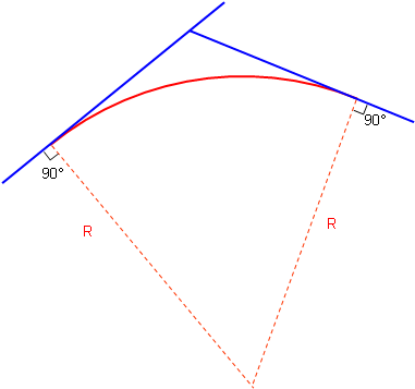
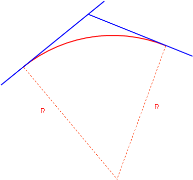
A simple tangent geometric curve is used to link the two lines. A curve is tangent to a line when its radius is perpendicular to the line, Figure C-1.

Figure C-1 Line-Curve Tangency Condition

 

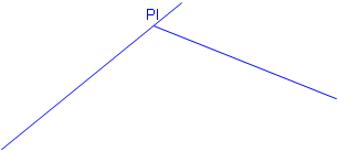
The two lines bounding the curve are generically referred to as tangents or tangent lines. The direction of a curve is either right or left based on the deflection direction between the tangents, Figures C-2 (a) and (b).

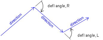(a) Deflection Angles	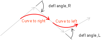(b) Curves
Figure C-2 Curve Direction

 

In roadway design horizontal geometry differs from vertical because a driver is responsible for guiding a vehicle from the first tangent to the second one. This requires turning a steering wheel changing the car's direction. Ideally this would be a smooth action to cause minimal discomfort: once into a curve, the steering angle would be maintained until the tangent is reached.

Two different mathematical arcs can be used for horizontal curves, either singularly or in combination: a circular arc and a spiral arc.

b. Circular arc

A circular arc has a fixed radius which means a driver doesn't have to keep adjusting the steering wheel angle as the car traverses the curve. It is a simple curve which is relatively easy to compute, Figure C-3.

Figure C-3 Circular Arc

 

Its primary disadvantage is that the constant curvature must be introduced immediately at curve's beginning. That means a driver would have to instantaneously change the steering wheel angle from 0° to full or the car would overshoot the curve. A similar condition exists ate the curves's end. The higher the vehicle speed and the sharper the curve, the more pronounced the effect.

c. Spiral arc

A spiral has a constantly changing radius, Figure C-4. At the spiral's beginning, its radius is infinite; as the vehicle progreeses into the curve, the spiral radius decreases. A spiral provides a more natural direction transition - the driver changes the steering wheel angle uniformly as the car traverses the curve.

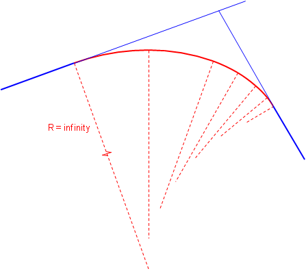Figure C-4 Spiral Arc

 

Attaching a second sprial with reversed radius change creates an entrance-exit spiral condition where the driver gradually increases then gradually decreases steering wheel angle, Figure C-5.

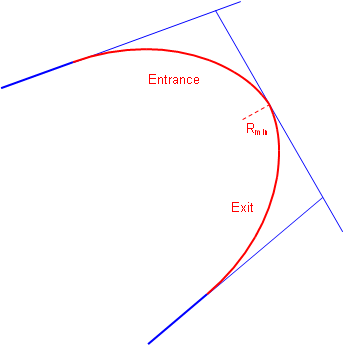Figure C-5 Combined Spirals

 

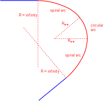
A circular arc can be combined with two spirals, Figure C-6.

Figure C-6 Spiralled Horizontal Curve

 

Combined spirals and spiralled horizontal curves, in conjunction with superelveation, help balance centrifugal forces. For a constant velocity, as the radius decreases the centrifugal force increases. A spiral allows superelevation to be introduced at a uniform rate allowing it to offset increasing centrifugal force. In theory, there exists an equilibrium velocity at which a vehicle could travel from one tangent through the spirals and curve to the second tangent safely even if the road were completely ice covered.

Railroad alignments typically use spiral horizontal curves because of their force balancing nature. Because of the wheel flange to rail connection, a train moving around a curve exerts a force directly to the rails (unlike a vehicle's tire-pavement connection which can devolve into a skid). A rail line laid out with a circular arc would shift to a spiral configuration after a train has run through it a number of time at transport speed.

The traditional disadvantage of a spiral is that it is complex to compute, although that has been largely negated by software. While still used for railways, in high speed highway design using long flat circular arcs minimizes the tangent to curve transition so spirals aren't as critical. They can be useful in low speed situations where there is a large direction transition. We'll examine spiral geometry and application in a later section.

2. Nomenclature; Components

a. Degree of Curvature

For any given set of tangents, there are an infinite number of circular arcs which can be fit between them. The arcs differ only in their radii which relates to their "sharpness." Consider the two arcs in Figure C-7:

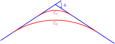Figure C-7 Different Arcs

 

Both curves must accommodate a total direction change of Δ but since C₁ is shorter it is sharper than C₂.

Degree of curvature is a traditional way of indicating curve sharpness. There are two different definitions of degree of curvature: arc and chord.

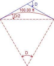
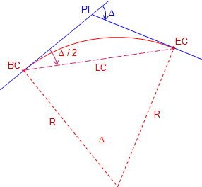
Arc definition, D_a, is the subtended angle for a 100.00 ft arc; Chord definition, D_c, is the subtended angle for a 100.00 ft chord, Figure C-8.

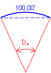(a) Arc Definition	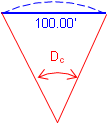(b) Chord Definition
Figure C-8 Degree of Curvature

 

Street and road alignments use the arc definition; chord definition is used for railroad alignments. For the remainder of this Chapter we will use the arc defintion and refer to it simply as D.

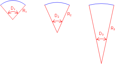
Degree of curvature is inversely proportional to radius: as D increases, R decreases, Figure C-9. The larger D is, the sharper the curve.

Figure C-9 D and R Relationship

 

Note the importance of 100.00 in both Degree of Curvature versions. This goes back to a standard tape length and stationing interval. However, in the metric system there is no convenient base equivalent of 100.00 ft. While design criteria was traditionally expressed in terms of D, it is more common today to instead use R which works for both the English and metric systems.

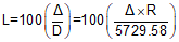
The relationship between D and R is expressed by Equation C-1.

Equation C-1

 

b. Curve Components; Equations

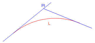
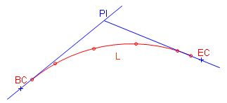
Figure C-10 shows a tangent circular arc with some basic components labeled. 

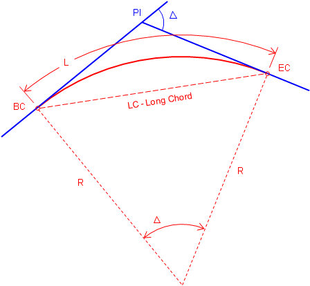Figure C-10 Basic Components of a Circular Arc

 

PI	Point of Instersection
BC	Begin Curve (aka: PC - Point of Curve; TC - Tangent to Curve)
EC	End Curve (aka: PT - Point of Tangent; CT - Curve to Tangent)
Δ	Defelction angle at PI; also the central angle of the arc
R	Arc radius
L	Arc Length
LC	Long Chord length

 

 Figure C-11 includes additional curve components.

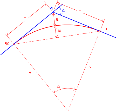Figure C-11 Additional Curve Components

 

T	Tangent distance
E	External distance - from PI to midpoint of arc
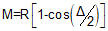
M	Middle ordinate - distance between midpoints of arc and Long Chord

 

Equations for the curve components are:

	Equation C-2
	Equation C-3
	Equation C-4
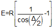	Equation C-5
	Equation C-6

 

Although it may look like it in Figure C-11, E and M are not equal.

c. Stationing

As mentioned in Chapter A, an alignment is stationed at consistent intervals from its beginning through its end. On a finished desgin, the stationing should be along the tangents and the fitted curves.

Traditionally, an alignment is stationed along the straight lines thru each PI, Figure C-12. Curve fitting comes later.

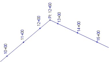Figure C-12 Stationing Along Tangents

 

A circular curve is fit and staked. The stationing along the tangents between curve ends would be replaced by the curve stations, Figure C-13.

There are two ways to get from BC to EC:

(1) Up and down the tangents, T+T
(2) Along the curve, L

The distance along the curve is shorter than up and down the tangents: L < T+T

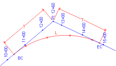Figure C-13 Curve Inserted

 

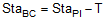
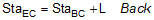
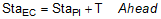
That means for a typical curve there are two stations for the EC:

One along the original tangents
One along the curve.

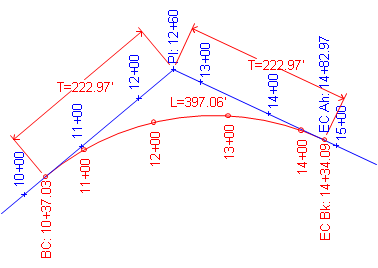Figure C-14 Stationing Along Curve

 

The EC station with respect to the original tangents is the EC Ahead. If we are standing on the EC and take a step ahead (up-station), we are on the tangent and its original stationing.

The EC station with respect to the curve is the EC Back. If we are standing on the EC and take a step back, we are on the curve and its stationing.

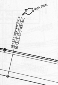
Chapter A mentioned that a station equation is used where one point has two stations. In this case we have a station equation at the EC: EC Sta Ahead = EC Sta Back. Figure C-15 is an example of a station equation indicator on a set of Wisconsin Dept of Trans highway plans.

Figure C-15 Station Equation Indicator

 

A station equation represents a stationing discontinuity. We know the distance between two alignment points is their stationing difference. However if the points are on each side of an EC, the discontinuity must be taken into account. For example, the distance between stations 13+00 and 16+00 on the alignment shown in Figure C-14 is normally 300.00 ft but there are 48.88 ft "missing" at the EC. The 48.88 ft is the difference between the Ahead and Back stations: (14+82.97) - (14+34.09) = 48.88 ft. So the correct distance from 13+00 to 16+00 is 251.12 ft.

With software, it is possible to avoid station equations by waiting until the curves are fitted before stationing the entire alignment. With computer assisted designs, the PIs could be computed positions, Figure C-16.

Figure C-16 Computed Tangents and PVI

 

A curve is then fit to the tangents, Figure C-17.

 

Figure C-17 A Curve is Fit

 

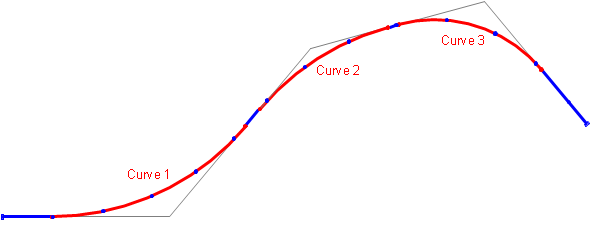
Then the alignment is stationed from its beginning to its end through the curves, Figure C-18. That way there are no station equations.

Figure C-18 Stationing Through Curve

 

So this latter method is simpiler and the one that should be used, right? Well, it does have some advantages, but it also has disadvantages. What happens if the alignment design must be changed at some point later in the process?

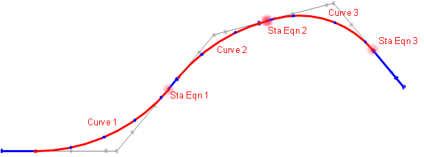
With traditional stationing, each curve has its own EC station equation. If one curve is altered, only its stationing is affected, no other stations on the alignment change, Figure C-19.

(a) Original Stationing with Station Equations

(b) Limited Stationing Changes with Curve Modification

Figure C-19 Alignment with Station Equations

 

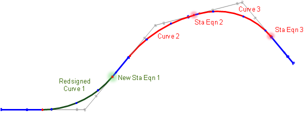
With continuous stationing, when a curve is altered it affects stations on it as well as all stations after it, Figure C-20.

(a) Original Continuous Stationing

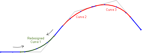(b) Stationing Changes on and after Modified Curve

Figure C-20 Alignment with Continuous Stationing

 

For example, if the redesigned curve is shorter, then all full (+00) station points after the curve increase. For example, 12+00 becomes 12+7.03, 13+00 becomes 13+07.03, etc. If the alignment is already staked then each stake could be renumbered or each could be each be moved back 7.03 feet. Hmm, odd stations or moving stakes.... Maybe station equations aren't so bad after all.

BC and EC stations are computed from the following formulae:

	Equation C-7
	Equation C-8
	Equation C-9

 

d. Example: Curve Components, Stationing

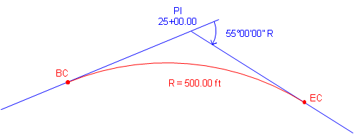
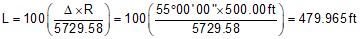
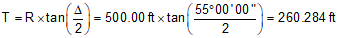
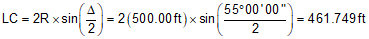
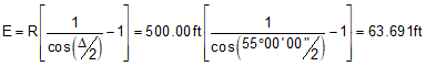
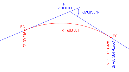
A PI is located at station 25+00.00. The deflection angle at the PI is 55°00'00" R. A 500.00 ft radius curve will be fit between the tangents.

Compute curve components and endpoint stations.

Start with a sketch:

Use Equations C-2 through C-6 to compute curve components (carry an additional digit to minimize rounding errors):

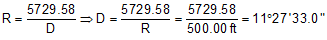
Compute degree of curvature using Equation C-1:

Use Equations C-7 through C-9 to compute endpoint stations:

 

3. Radial Chord Method

a. Circular Geometry

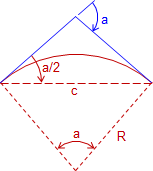
For any circular arc, the angle between the tangent at one end of the arc and the chord is half the arc's central angle, Figure C-21.

Figure C-21 Deflection angle

 

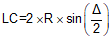
 Angle a/2 is the deflection angle from one end of the arc to the other. The chord's length is computed from:

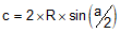Equation C-10

 

In terms of the degree of curvature, Figure C-22: 

Figure C-22 Full station deflection angle

 

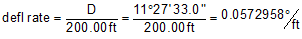
The deflection angle for a full station is half the degree of curvature. Since the deflection angle is D/2 and it occurs over a 100.00 ft, the deflection rate can be computed from:

Equation C-11

 

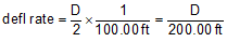
Extending this geometry to the entire curve, Figure C-23, the total deflection angle at the BC from the PI to the EC is Δ/2.

Figure C-23 Deflection angle for entire curve

 

Since the deflection angle occurs across the curve's length, the deflection rate can also be written as Equation C-12.

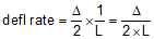Equation C-12

 

b. Radial chords

One way to stake a horizontal curve is by the radial chord method, Figure C-24.

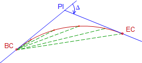Figure C-24 Radial chord method

 

An instrument is set up on the BC and the the PI is used as a backsight. Then to stake each curve point, an angle is turned and distance measured. For each curve point, we need to compute its deflection angle from the tangent and chord distance from the BC.

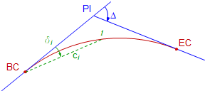
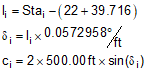
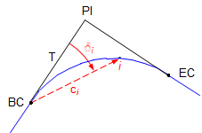
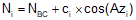
The deflection angle to any point i on the curve, Figure C-25, can be computed from Equation C-13.

Figure C-25 Deflection angle and radial chord

  

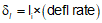Equation C-13

 

l_i is the arc distance to the point from the BC and is computed using Equation C-14.

Equation C-14

 

Equation C-10 can be re-written using the deflection angle:

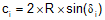Equation C-15

 

Using Equations C-13 to C-15, the deflection angle and distance to any curve point from the BC can be computed.

 

c. Example

Determine the radial chord stakeout data at full stations for the example from Section 2.d.

Summary of given and computed curve data:

Δ = 55°00'00"	R = 500.00 ft
D = 11°27'33.0"	L = 479.965 ft	T = 260.284 ft
LC = 461.749 ft	E = 63.691 ft	M = 56.494 ft

Point	Station
PI	25+00.00
BC	22+39.716
EC	27+19.681 Bk = 27+60.284 Ah

Use Equation C-11 to compute the curve's deflection rate:

Set up Equations C-13, C-14, and C-15 for the curve:

Set up the Curve Table: 

Curve Point		Arc dist, li, (ft)	Defl angle,δi	Radial chord, ci
EC	27+19.681 Bk
	27+00
	26+00
	25+00
	24+00
	23+00
BC	22+39.716

 

Solve the three equations for each curve point and record the results in the table.

At 22+39.716, we're still at the BC so all three entries are zero.

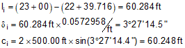
At 23+00:

And so on until the table is complete.

Curve Point		Arc dist, li, (ft)	Defl angle,δi	Radial chord, ci
EC	27+19.681 Bk	479.965	27°30'00.0"	461.748
	27+00	460.284	26°22'20.4"	444.203
	26+00	360.284	20°38'33.9"	352.540
	25+00	260.284	14°54'47.4"	257.355
	24+00	160.284	9°11'01.0"	159.599
	23+00	60.284	3°27'14.5"	60.248
BC	22+39.716	0.000	0°00'00.0"	0.000

 

Math checks:

Arc distances between successive full stations differ by 100.00 ft.

At the EC:

Arc distance should equal the curve length

Defl angle should equal Δ/2

Radial chord should equal Long Chord

The difference between deflection angles at successive full stations should be D/2.

These checks have been met.

Remember that we carried additional decimal places to minimize rounding errors. Rounding can become quite pronounced for long flat curves so computation care must be exercised. Once the table has been computed, the final values can be shown to reasonable accuracy levels. For example, distances can be shown to 0.01 ft and deflection angles to 01".

d. Summary

Computing and staking curve points by the radial chord method is simple and straightforward. Using the curve equations, any point on the curve can be computed and staked, not just those included in the curve table.

However, in the field, it may not be the most efficient way to stake a curve using modern instrumentation, particularly with long curves which may have chords thousands of feet long at very small deflection angles. Most contemporary survey computations and fieldwork use coordinates giving greater stakeout flexibility. While the radial chord method may not be used for stake out, it is well adapted to coordinate computations as we'll see in the next section.

4. Curves and Coordinates

a. Coordinate Equations

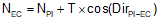
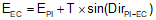
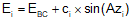
Equations C-16 and C-17 are general equations for computing coordinates using direction and distance from a known point, Figure C-26.

		Equation C-16
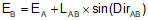		Equation C-17

 

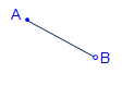Figure C-26. Coordinate Computation

 

Direction (Dir) may be either a bearing or azimuth.

Curve point coordinates can be computed using these equations from a base point. Since the radial chord method uses the BC as one end of all the chords, it can also be used as the base point for coordinate computations.

b. Computation Process

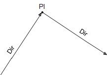
Assuming we start with the tangents and PI, then fit a curve, the general process is as follows:

Figure C-27		The original tangent lines have directions; PC has coordinates.
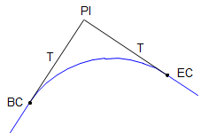
Figure C-28		A curve is fit to the tangents. End points are at distance T from the PI along the tangents.
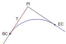
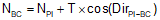
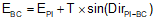
Figure C-29		Compute coordinates of BC using back-direction of the tangent BC-PI and T.       Equation C-18   Equation C-19
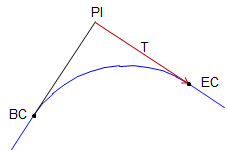
Figure C-30		Compute coordinates of EC using direction of the tangent PI-EC and T. These will be use for a later math check.       Equation C-20     Equation C-21
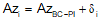
Figure C-31		Use a curve point's deflection angle to compute the direction if its radial chord from the BC.       Equation C-22    δ is positive for right deflections, negative for left. Using the direction and chord length, compute the point's coordinates.       Equation C-23      Equation C-24

 

c. Example

Continuing with the previous example problem.

Summary of given and computed curve data: 

Δ = 55°00'00"	R = 500.00 ft
D = 11°27'33.0"	L = 479.965 ft	T = 260.284 ft
LC = 461.749 ft	E = 63.691 ft	M = 56.494 ft

 

Point	Station
PI	25+00.00
BC	22+39.716
EC	27+19.681 Bk = 27+60.284 Ah

 

 

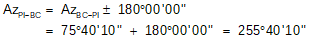
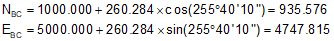
Additional information: Azimuth of the initial tangent is 75°40'10"; coordinates of the PI are 1000.00 N, 5000.00' E.

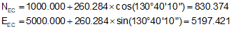
Compute coordinates of the BC:

Compute the coordinates of the EC:

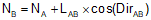
Set up Equatons C-21 through C-24 for this curve.

This is the Radial Chord table computed previously:

Curve Point		Arc dist, li, (ft)	Defl angle,δi	Radial chord, c
EC	27+19.681 Bk	479.965	27°30'00.0"	461.748
	27+00	460.284	26°22'20.4"	444.203
	26+00	360.284	20°38'33.9"	352.540
	25+00	260.284	14°54'47.4"	257.355
	24+00	160.284	9°11'01.0"	159.599
	23+00	60.284	3°27'14.5"	60.248
BC	22+39.716	0.000	0°00'00.0"	0.000

 

 Add three more columns for direction and coordinates:

Curve Point		Azimuth, Azi	North, Ni	East, Ei
EC	27+19.681 Bk
	27+00
	26+00
	25+00
	24+00
	23+00
BC	22+39.716

 

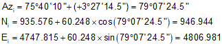
Complete the table using the three equations for this curve

At 22+39.716, we're still at the BC so the coordinates don't change.

At 23+00:

At 24+00:

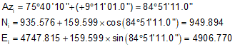
and so on for the rest of the curve points.

The completed curve table is: 

Curve Point		Azimuth, Azi	North, Ni	East, Ei
EC	27+19.681 Bk	103°10'10.0	830.375	5197.419
	27+00	102°02'30.4"	842.904	5182.244
	26+00	96°18'43.9"	896.816	5098.218
	25+00	90°34'57.4"	932.959	5005.157
	24+00	84°51'11.0"	949.894	4906.770
	23+00	79°07'24.5"	946.944	4806.981
BC	22+39.716	75°40'10"	935.576	4747.815

 

Math check: the coordinates computed for the EC in the table should be the same as the EC coordinates computed from the PI. Within rounding error, that's the case here.

d. Summary

The radial chord method lends itself nicely to computing curve point coordinates. The computations are not complex, although they are admittedly tedious.

Once coordinates are computed, field stakeout is much more flexible using Coordinate Geometry (COGO).

 

Section 5. Chord Definition

a. General

Recall from Section 2 there are two definitions for degree of curvature, Figure C-32.

a. Arc Definition	b. Chord Definition
Figure C-32 Degree of Curvature

Arc definition is the central angle for a 100.00 ft arc; chord is for a 100.00 ft chord.
Since the geometry is slightly different, the mathematical relationship between R and D_c is Equation C-25.

Equation C-25

Equations C-3 through C-6 for T, LC, E, and M can be used with no changes.

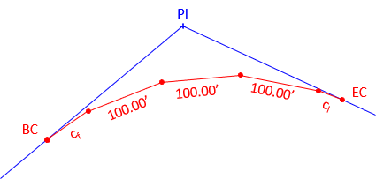
Equation C-2 for L does not yield the total arc length of the curve from the BC to EC. It returns the sum of the subchords, Figure C-33 and Equation C-26.
 

Figure C-33 Sum of the Chords

 

Equation C-26

 Where:

cf	first partial chord (<100.00 ft)
n	number of full 100.00 ft chords on the curve
cl	last partial chord (<100.00 ft)

 

b. Stationing

The same equations are used to compute endpoint stationing for arc and chord definition curves.

	Equation C-27
	Equation C-28
	Equation C-29

 
A notable difference from the arc definition is that curve stationing is along the chords, not the arcs.
 

c. Radial Chord Deflection Method

Because stationing is through the chords, deflection angles to curve points are can be computed by adding incremental deflection angles. The radial chord to each curve point is determined using Equation C-15.

First partial chord, c_f

c_f is the difference between the first full curve station and the BC station.
The central angle and incremental deflection angles are:

	Equation C-30
	Equation C-31

Last partial chord, c_l:

c_l is the difference between the last full curve station and the EC Back station.
The central angle and incremental deflection angles are:

	Equation C-32
	Equation C-33

 
Nominal chord

The chord between adjacent full stations is 100.00 ft.
The incremental deflection angle is:

Equation C-34

Starting with the first incremental deflection angle, the procedure to compute total deflection angle to curve points is:

 

d. Example Problem

PI Station is 59+45.00, Δ angle is 30°00'00", a 7°00'00" degree of curvature (chord def) will be used.
Compute the curve table.

(1) Curve components

(2) Stationing

(3) Incremental deflection angles

first partial chord

last partial chord

nominal chord

(4) Curve Table

Set up table with stations and incremental deflection angles

	Sta	Inc Defl	Total Defl	Radial Chord
EC Bk	61+54.115	1°53'39"
	61+00	3°30'00"
	60+00	3°30'00"
	59+00	3°30'00"
	58+00	2°36'21"
BC	57+25.544	0°00'00

Compute total deflection angle by adding incremental deflection angles

	Sta	Inc Defl	Total Defl	Radial Chord
EC Bk	62+65.715	1°53'39"	15°00'00"
	62+00	3°30'00"	13°06'21"
	61+00	3°30'00"	9°36'21"
	60+00	3°30'00"	6°06'21"
	59+00	2°36'21"	2°36'21"
BC	58+37.174	0°00'00	0°00'00"

Total deflection angle to EC is 30°00'00"/2 = 15°00'00"  check

 Compute radial chord to curve point using:

	Sta	Inc Defl	Total Defl	Radial Chord
EC Bk	62+65.715	1°53'39"	15°00'00"	423.96
	62+00	3°30'00"	13°06'21"	371.43
	61+00	3°30'00"	9°36'21"	273.34
	60+00	3°30'00"	6°06'21"	174.42
	59+00	2°36'21"	2°36'21"	74.47
BC	58+37.174	0°00'00	0°00'00"	0.00

Radial chord to EC is 423.96' = LC  check

e. Arc Length

Should it be needed, the arc length, L_A, from the BC to the EC, can be computed using Equation C-35.

Equation C-35

Δ_r is the Δ angle in radians, Equation C-36.

Equation C-36