This supplemental material is provided for the curious. Understanding it isn't necessary to perform vertical curve computations. You may safely ignore it, but now that you know it's here, you'll eventually be back.
A convenient way to look at a vertical curve and derive its equation is by examining its Family of Curves. These relate the vertical curve to its grade and grade change behavior.
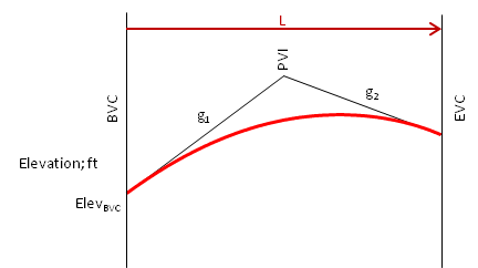
Starting with a crest vertical curve fit between positive incoming and negative outgoing grades, Figure 1.
 |
| Figure 1 Crest Curve |
The curve represents elevations at different horizontal distances from the BVC.
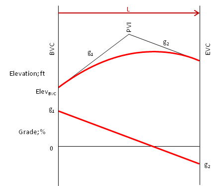
Remember that for a vertical curve, the grade change rate, k, is constant. That means the grade changes linearly from g1 to g2. If we plot this and add it to Figure 1 we get Figure 2.
 |
| Figure 2 Adding Grade |
This graph shows the grade of the line tangent to the curve at different distances from the BVC.
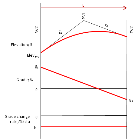
Grade change rate, k is constant, Equation 1, and it can also be plotted. For a crest curve k is negative.
 |
Equation 1 |
Plotting and adding k to Figure 2 gives us Figure 3.
 |
| Figure 3 Adding Grade Change Rate |
No matter where we are on the curve, k is the same. For this crest curve, k is negative causing the tangent grade to decrease along the curve length.
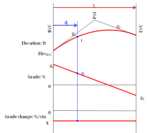
This set of graphs is referred to as the Family of Curves. They graphically represent the vertical curve calculus. Starting with the parabolic curve, its first derivative is the grade curve (slope), its second derivative is k (max/min).
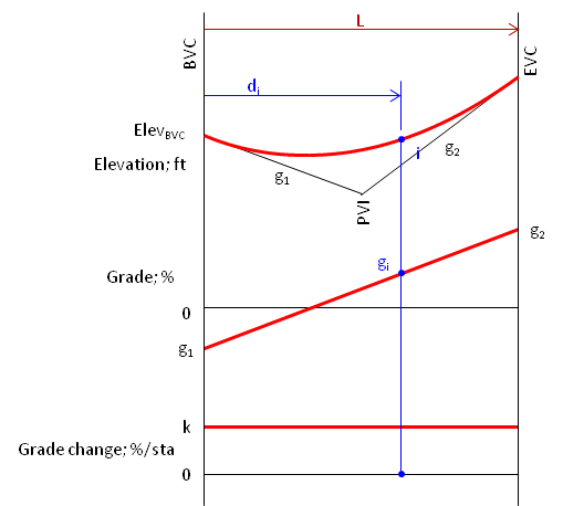
How can we use these? Back to calculus: an area under a lower curve represents changes in the next higher curve. For example, consider point i at distance di from the BVC, Figure 4.
 |
| Figure 4 Family of Curves |
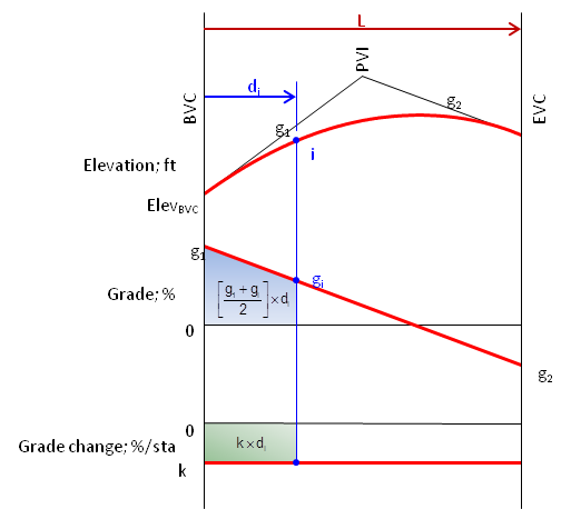
The grade at point i, gi, is equal to g1 plus the area under the grade change curve at the distance di, Figure 5.
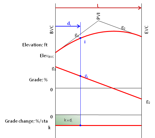 |
| Figure 5 Grade at Distance i |
 |
Equation 2 |
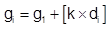
The elevation at point i is equal to the elevation of the BVC plus the area under the grade curve at the distance di, Figure 6.
 |
| Figure 6 Elevation at Distance i |
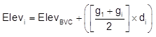 |
Equation 3 |
Combining Equations 1 - 3 and simplifying, we get the Curve Equation, Equation 4:
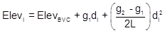 |
Equation 4 |
A sag vertical curve has a similar Family of Curves, Figure 7.
 |
| Figure 7 Sag Family of Curves |
The curve relationships are the same as those for a crest curve. The primary difference is that k is positive causing the tangent grade to increase along the curve length.
Side note:
This set of curves is not unique to vertical curves in surveying; it also applies to structures. From bottom to top, the curves represent uniform loading on a beam, shear, and moment. Neat, huh?