4. Example
Adjust the level circuit of Chapter C shown in Figure D-2.
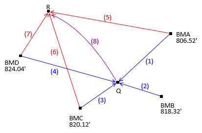 |
| Figure D-2 Level Circuit |
| Obs | Line | dElev | Obs | Line | dElev | |
| 1 | BMA-Q | +8.91 | 5 | BMA-R | -3.56 | |
| 2 | BMB-Q | -2.92 | 6 | BMC-R | -17.12 | |
| 3 | BMC-Q | -4.67 | 7 | BMD-R | -21.10 | |
| 4 | BMD-Q | -8.66 | 8 | Q-R | -12.47 |
(1) Observation Equations
Use Equation D-4 as the initial observation equation format, then rearrage to place the unknowns on the left side, constants and residuals on the right.
| Equation D-43 |

(2) Set up Matrices

(3) Solve Unknowns: [U] = [Q] x [CTK]
[CT] x [C]

[CT] x [K]

Invert [CTC] to get [Q]

[Q] x [CTK]

These are the same elevations as in the Direct Minimization method.
(4) Adjustment Statistics
Residuals: [V] = [CU] - [K]

Compute So

![]()
Standard deviations for points Q and R elevations using Equation D-2

Adjusted observations

Adjusted observation uncertainties using Equation D-7.
Obs 1
First row of [C] and first column of [CT].

Because rows 1-4 of the C matrix are the same, all four observations will have the same expected error.
Ditto for observations 5-7
Obs 5
Fifth row of [C] and fifth column of [CT].

Obs 8
Eighth row of [C] and eighth column of [CT].

Outside of having the same [C] coefficients, why do observations 1-5 have the same expected errors? Because each connects a benchmark to the adjusted point Q (that's why they have same rows in [C]). The only error affecting those observations is point Q's. Similarly, observations 5-7 are only affected by point R. Only the eighth observation has uncertainties at both ends.
(5) Adjustment Summary
Degrees of freedom: DF = 8-2 = 6
Std Dev Unit Wt: So = ±0.028
Adjusted elevations
| Point | Elevation | Std Dev | |
| Q | 815.418 | ±0.013 | |
| R | 802.962 | ±0.014 |
Adjusted observations
| Line | Adj Obs | SE |
| BMA-Q | 8.898 | ±0.013 |
| BMB-Q | -2.902 | ±0.013 |
| BMC-Q | -4.702 | ±0.013 |
| BMD-Q | -8.622 | ±0.013 |
| BMA-R | -3.558 | ±0.014 |
| BMC-R | -17.158 | ±0.014 |
| BMD-R | -21.078 | ±0.014 |
| Q-R | -12.456 | ±0.017 |