D. Multi-Center Horizontal Curves
1. General
A multi-center curve consists of two or more back-to-back curves that are tangential. The simplest consists of two curves either in the same direction (compound) or opposite directions (reverse), Figure D-1.
 |
 |
| a. Compound curve | b. Reverse curve |
| Figure D-1 Multi-center curves |
|
Multi-center curves provide greater design flexibility. For example, Figure D-2 shows a typical cloverleaf freeway interchange.
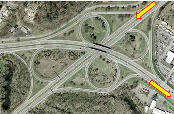 |
| Figure D-2 Cloverleaf interchange |
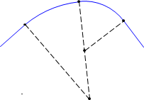
To travel southeast, southwest-bound traffic changes direction approximately 280° using the southwestern loop. This is accomplished using a flat curve for initial deceleration, followed by sharper curves for most of the direction change, and finally shallower acceleration curves. Figure D-3 shows the southwestern loop with overlaid circular arcs.
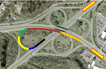 |
| Figure D-3 Multiple curves |
Using a multi-center curve makes the interchange more space efficient; consider how much area would be needed for a single radius curve in this situation.
A reverse curve also provides design flexibility, particularly in tight areas.
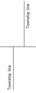
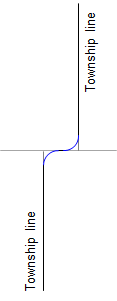
For example, in Public Land Survey (PLS) states, north-south Township lines were offset along Standard Parallels to account for meridian convergence, Figure D-4a. Roads commonly followed Section and Township lines. At an offset Township line, a sharp left turn shortly after a sharp right turn was perfectly acceptable at horse drawn wagon speed, Figure D-4b. As vehicle speeds increased, flatter curves were necessary but had to fit between the Township line segments. This could be done using a reverse curve, Figure D-4c.
 |
 |
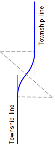 |
| a. Convergence offset | b. Low speed curves | c. High speed curves |
| Figure D-4 Offset Township lines |
||
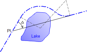
A reverse curve can also be used to work an alignment around an obstruction. Figure D-5 shows what, were it not for the presence of a lake, would be a simple curve situation .
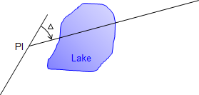 |
| Figure D-5 Obstruction |
Neither a long nor short radius single curve will miss the lake. However, a curve to the right could be fit to an extension of the incoming tangent followed by a curve to the left to meet the original outgoing tangent, Figure D-6.
 |
| Figure D-6 Working around obstruction |
If multi-center curves are so flexible, why don't we see more of them?
Primarily because of the curvature change at each curve-to-curve transition.
On a simple curve, once the driver sets the steering wheel angle, it is maintained through the entire curve. A multi-center curve requires a steering wheel angle change at the beginning of each curve. Except for a reverse curve, it may not be visually apparent where one curve ends and the next begins. This makes it easy to over- or under-shoot successive curves.
Traveling around a circular arc introduces centrifugal force which pushes the vehicle (and its occupants) to the outside of the curve. The sharper the curve or the higher the speed, the greater the force. One way to offset this centrifugal effect is to use superelvation - pavement cross-slope inclination. As a vehicle traverses differing radii curves, different superelevation rates are needed. Superelevation change should be introduced gradually or passengers may feel like they are being tossed to the side. This is more pronounced with a large radii difference from one curve to the next. On a reverse curve the condition can be worse since the cross-slope direction must be changed.
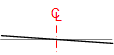
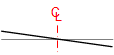
Figure D-7 shows a three-center curve system with 5 section view labels.
 |
| Figure D-7 Three-center curve |
Table D-1 depicts the steering wheel angle and superelevation at each section view going through the curve system.
| Table D-1 | ||
| Section | Steering Wheel | Superelevation |
| A-A | 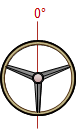 |
 |
| B-B | 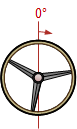 |
 |
| C-C | 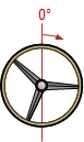 |
 |
| D-D | 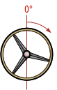 |
 |
| E-E | 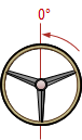 |
 |
Note that the greatest wheel angle and superelvetion occur on the third curve and must be removed entirely when the exit tangent is reached. That abrupt change could cause safety and comfort issues.
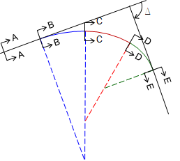
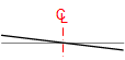
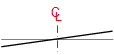
A reverse curve provides an additional chanllenge, Figure D-8 and Table D-2.
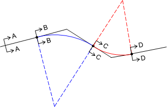 |
| Figure D-8 Reverse Curve |
| Table D-2 | ||
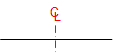
| Section | Steering Wheel | Superelevation |
| A-A | 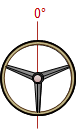 |
 |
| B-B | 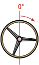 |
 |
| C-C | 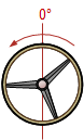 |
 |
| D-D | 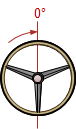 |
 |
At the point of reverse curvature, the steering angle must be changed to the other side. The superelevation also changes direction so the vehicle is "rolled" from one side to the other. Coupled with superelevation, the centrifugal force changes direction. All-in-all quite a bit of stuff going on, especially when the vehicle is cruising along at a good rate.
So while multi-center curves provide greater design flexibility, they do have drawbacks. particularly in high speed situations. Except for special cases such as interchanges, their use should be limited to lower speeds with reasonable radii differences.
2. Compound curve
a. Nomenclature
Starting with two tangent lines intersecting at a PI, a compound curve is fit between them, Figure D-9.
 |
| Figure D-9 Compound curve |
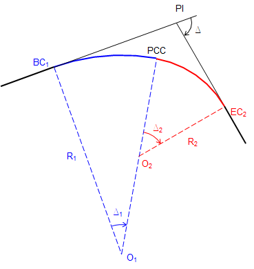
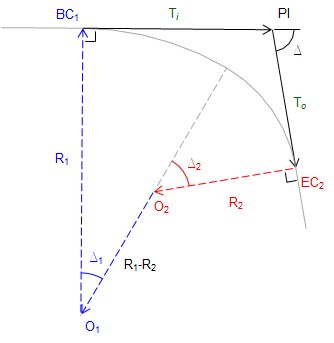
Figure D-10 shows major parts of the compound curve.
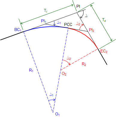 |
| Figure D-10 Compound curve parts |
The PCC (Point of Curve to Curve) is the EC of the first curve and BC of the second. A tangent line at the PCC intersects the incoming tangent at the PI1 and the outgoing tangent at PI2.
Ti is the distance from the BC1 to the PI; To the distance from the PI to the EC2.
There are seven parts to a compound curve: Ti, To, R1, R2, Δ1, Δ2, and Δ. Because the tangents deflect Δ at the PI and the compound curve transitions from the incoming to the outgoing tangent:
| Δ = Δ1+ Δ2 | Equation D-1 |
That means there are six independent parts. For a unique solution four parts must be fixed, including at least one angle and at least two distances.
Because they share a point (PCC) and tangent line, once all six parts are determined, the compound curve can be computed as two simple curves, Figure D-11. Individual curve attributes can be computed using the single curve equations in Chapter C.
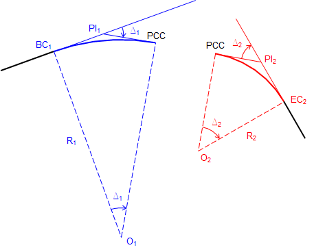 |
| Figure D-11 Two simple curves |
Depending on which parts are initially fixed, there are different ways to compute the remaining parts.
One way is solving the vertex triangle, Figure D-12, created by the three PIs.
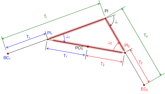 |
| Figure D-12 Vertex triangle |
Another method is to use a closed loop traverse through points O1-BC1-PI-EC2-O2, Figure D-13.
 |
| Figure D-13 Traverse method |
The direction of one line is assumed to be in a cardinal direction and the others written in terms of 90° angles and Δs. Distances are Rs and Ts. Latitudes and departures are computed, summed, are set equal to zero to force closure. This results in two equations in two unknowns which can then be simultaneously solved.
b. Examples
(1) Example 1
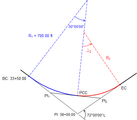
A PI is located at station 38+00.00 with a left deflection of 72°00'00"L. The compound curve begins at sta 33+50.00. The first curve has a 700.00 ft radius and 30°00'00" central angle.
Determine the radius and central angle of the second curve and the length of both curves.
Sketch:
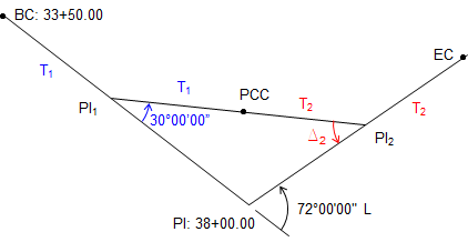
We'll try a vertex triangle solution. Isolate the triangle and label the tangents:
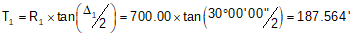
Since we have the radius and central angle of the first curve, we can compute its tangent:
Compute Δ2 using Equation D-1

Determine the distance from the PI1 to the PI which is a side of the triangle.
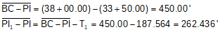
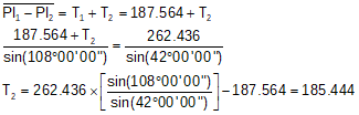
The distance between PI1 and PI2 is the sum of the curve tangents. Using the Law of Sines and the known T1, we can compute T2.
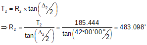
Using T2 and Δ2, R2 can be determined.
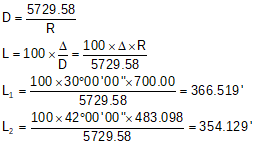
Finally, compute each curve's length.
(2) Example 2
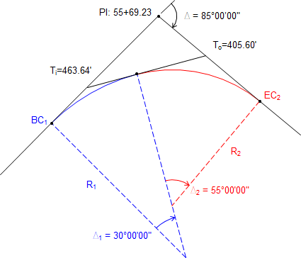
A PI is located at 55+69.23 with a deflection angle between tangents of 85°00'00"R. The compound curve must begin 463.64 ft before the PI and end 405.60 ft after. Central angles of the two curves are 30°00'00" and 55°00'00", respectively.
Determine the radius of each curve,
Sketch:
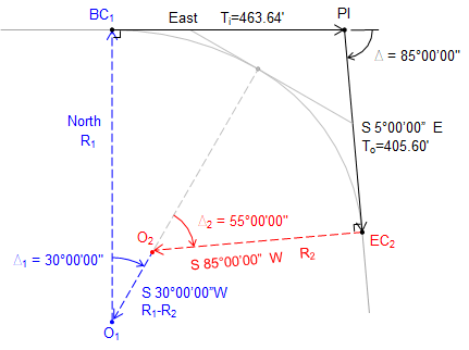
Because we only have angles of the vertex triangle with no distances (and insufficient given data to compute any), the curve system can't be solved that way. Instead, we will use the traverse method.
To start, the curve system is rotated to make the initial radial line run North. Then using right angles and Δs, bearings (or azimuths) of the other lines can be determined.
Updated sketch with bearings:
Compute Latitudes and Departures:
| Line | Bearing | Length | Latitude | Departure |
| O1-BC1 | North | R1 | R1 | 0.00 |
| BC1-PI | East | 463.64 | 0.00 | 463.64 |
| PI-EC2 | S 5°00'00"E | 405.60 | -405.60 x cos(5°00'00") | +405.60 x sin(5°00'00") |
| EC2-O2 | S 85°00'00"W | R2 | -R2 x cos(85°00'00") | -R2 x sin(85°00'00") |
| O2-O1 | S 30°00'00"W | R1-R2 | -(R1-R2) x cos(30°00'00") | -(R1-R2) x sin(30°00'00") |
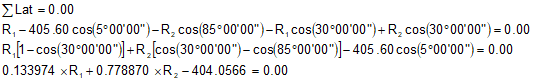
Sum and reduce the Latitudes:
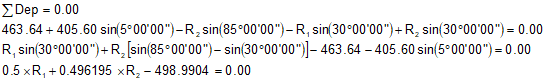
Sum and reduce the Departures:
We have two equations with unknowns R1 and R2. Solve them simultaneously. We'll use substitution.
Solve the Latitude summation for R1
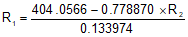
Substitute the equation for R1 in the Departures summation and solve R2:
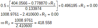
Solve R1:
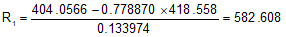
With R1 and R2 computed, we have two geometric attributes for each curve. Using Chapter C. Horizontal Curves equations, their remaining attributes can be determined.
c. Stationing
As with a single curve, there are two paths to the EC from the BC. One goes up and down the original tangents, the other along the curves. Whether a station equation is used at the EC depends on how the entire alignment is stationed. Refer to the Station Equation discussion in Chapter C. Horizontal Curves.
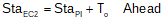
Equations to compute the curves' endpoints are:
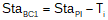 |
Equation D-2 | |
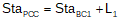
 |
Equation D-3 | |
 |
Equation D-4 | |
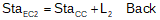 |
Equation D-5 |
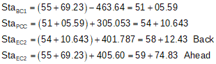
The stationing for Example (2) is:
e. Radial stakeout
Each curve's table is computed as described in Chapter C. Horizontal Curves.
Following are radial chord tables for each curve in Example (2) (computations aren't shown).
| Curve 1 | |||
| Sta | Defl ang | Chord | |
| EC | 54+10.64 | 15º00'00" | 301.58 |
| 54+00 | 14º28'36" | 291.29 | |
| 53+00 | 9º33'34" | 193.51 | |
| 52+00 | 4º38'32" | 94.31 | |
| BC | 51+05.59 | 0º00'00" | 0.00 |
| Curve 2 | |||
| Sta | Defl ang | Chord | |
| EC | 58+12.43 | 27º30'00" | 386.54 |
| 58+00 | 26º38'57" | 375.47 | |
| 57+00 | 19º48'17" | 283.63 | |
| 56+00 | 12º57'37" | 187.77 | |
| 55+00 | 6º06'57" | 89.109 | |
| BC | 54+10.64 | 0º00'00" | 0.00 |
Stakeout procedure
Measure Ti and To from the PI along the tangents to set the BC1 and EC2.
Stake Curve 1
Setup instrument on BC1.
Sight PI with 0º00'00" on the horizontal circle.
Stake curve points using the curve table.
Stake Curve 2
Setup on PCC
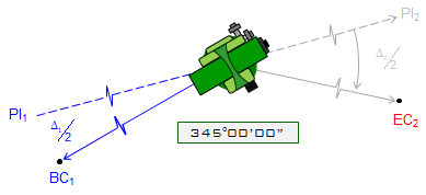
Sight BC1 with -(Δ1/2) = -15º00'00"=345°00'00" on the horizontal circle, Figure D-14a.
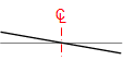
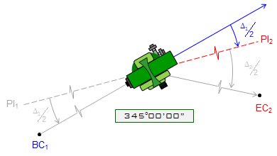
Inverse the scope to sight away from the BC1, Figure D-14b.
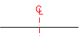
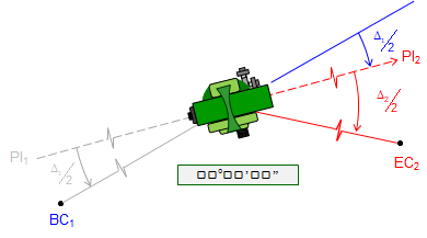
Rotating right to a horizontal angle of 0º00'00" orients instrument tangent to the curves at the PCC, Figure D14c.
Stake curve points using the curve table.
Last point should match the previously set EC2.
 |
|
a. Sight BC1 with -(Δ1/2) reading |
 |
| b. Inverse telescope |
 |
| c. Rotate to 00°00'00" |
| Figure D-14 Orienting at PCC |
3. Reverse curve
a. General
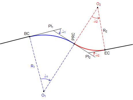
A reverse curve consists of two consecutive tangent curves with radius points on opposite sides of the center line. Figure 15 shows basic nomenclature and parts.
 |
| Figure D-15 Nomenclature |
The PRC is the Point of Reverse Curvature, and is the EC of the first curve and BC of the second.
The distance from PI1 to PI2 is T1 + T2. Because of this relationship, as soon as one curve's geometry is fixed, so is the other's. This makes a reverse curve generally easier to compute than a compound curve.
Once the geometry of both curves are fixed, they can be computed as individual simple curves.
b. Stationing
Stationing can be a little confusing since there can be a station equation at both the PRC and EC of the second curve. Usually, if a stationing is maintained along the tangents, then a station equation only appears at the end of the reverse curve.
To compute stationing:
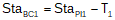 |
Equation D-6 | |
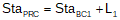 |
Equation D-7 | |
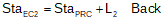 |
Equation D-8 | |
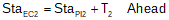 |
Equation D-9 |
b. Example
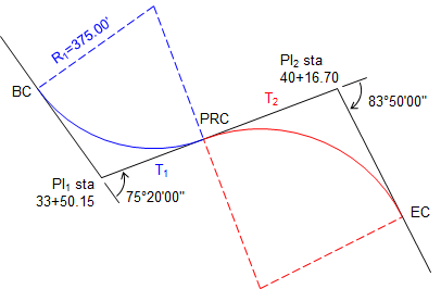
For a reverse curve, the first PI is at 33+50.15 with a 75°20'00"L deflection angle and second PI is at 40+16.70 with a 83°50'00"R deflection angle.
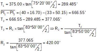
The first curve has a 375.00' radius. Determine the radius of the second curve.
Sketch:
Ta-daa!