2. Statistics
How many measurements must be made to be statistically significant? Good question, and not an easy one to answer. We know that at least three measurements should be made in order to trap mistakes, but three is pretty light. Once we introduce some analysis equations, we'll be able to make some predictions. For now, we'll use a small measurement set to explain some terms and statistical analyses.
Our sample measurement set is: 45.66 45.66 45.68 45.65
a. Discrepancy
The difference between any two measurements of the same quantity.
Example: the discrepancy between the highest and lowest measurements is 0.03
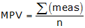
b. Most Probable Value (MPV)
This is a fancy way of saving average or mean. In simplest form, it's the measurement sum divided by the number of measurements.
 |
Equation F-1 |
|
MPV: most probable vlaue |
|
Example: MPV = (45.66+45.66+45.68+45.65)/4 = 45.662
In analyses where mixed-quality measurements are combined the MPV might be called a “weighted average.” This takes into account quality variations giving higher consideration to better quality measurements. For our purposes, measurements will be made using consistent instrumentation and procedures so we will use an unweighted average (also called a unit weight average).
c. Residual (v)
The difference between a measurement and the MPV. This is like a discrepancy except it’s always compared against the MPV.
Example: Residual of the first measurement is 45.66-45.662 = -0.002
It doesn't really matter if the MPV is subtracted from the measurement or vice versa since we will ultimately square each so the mathematical sign goes away. Just be consistent: (measurement-MPV) or (MPV - measurement).
d. Normal Distribution Curve
Computing all the residuals and plotting their frequency results in a bell-shaped curve, Figure F-1. The curve is symmetric with smaller residuals more frequent and grouped closer to the MPV. The curve is asymptotic: it approaches the x-axis but never touches it.
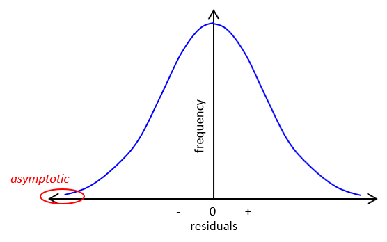 |
| Figure F-1 Normal Distribution Curve |
Of course with only four measurements in this example, ours would be a pretty sorry looking bell. Just like flipping the coin, as you approach an infinite number of measurements your graph becomes a smooth curve.
e. Standard Deviation
On both sides of the curve is an inflection point: where the curve changes from convex to concave. These occur at ±σ along the x-axis, Figure F-2.
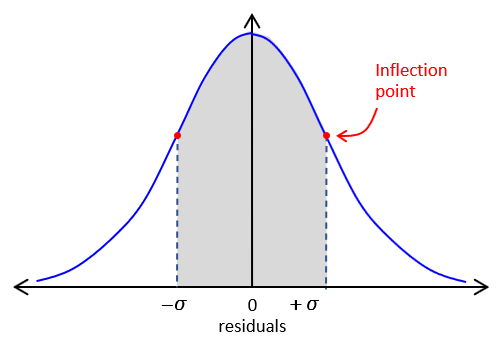 |
| Figure F-2 Standard Deviation |
To compute the standard deviation:
 |
Equation G-2 | |
| σ: standard deviation v: residual n: number of measurements |
||
You’ll also see another form of the equation:
 |
Equation F-3 |
What's the difference? This is a little over-simplified, but basically:
Equation F-2 is used for a subset of all the data (sample set)
Equation F-3 is used with an entire data set (entire population)
Equation F-3 is referred to as the Standard Error. It's used when an entire data set us available for measurement. Standard deviation is used when it's not practical to analyze all the data.
Example:
To determine the compressive strength of concrete that will be used to build a structure, test cylinders of the fresh concrete are poured and then destructively tested at 7, 30, and 365 days. To determine the concrete's average strength and its standard error, all the concrete would be tested (entire population) leaving nothing with which to build the structure. That is neither practical nor economically feasible. Instead, random samples are taken from batch mixes and tested. From this sample subset we determine the average strength and its standard deviation.
In surveying, we attempt to determine an unknown quantity by measurement. The entire population can only be attained with an infinite number of measurements. We are limited to a finite number of measurements - we collect a sample of the entire population. So to analyze our measurements, we use the standard deviation from Equation G-2. The larger the sample set, the better the statistical analysis.
Adding to the confusion, some texts use σ for standard deviation and S for standard error while others use S for standard deviation and σ for standard error. Whatever it's called, remember: in measurement science we work with a sample set so always use (n-1) in the denominator.
Note that as n increases, the difference between Equations F-2 and F-3 decreases. When n hits infinity, division by either infinity or (infinity-1) makes little difference.
Anyway, back to standard deviation, Equation F-2...
This area bounded by ±σ and the curve is ~68.3% of the total area under the entire normal distribution curve. What that means is ~68% of our measurements fall within ±σ of the MPV.
Standard deviation is an indicator of the measurement set's precision: the smaller the standard deviation, the smaller the data spread, the better the precision. Figure F-3 demonstrates this for two different measurement sets.
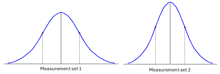 |
| Figure F-3 Standard Deviation and Precision |
f. Confidence Interval (CI)
A confidence interval is the degree of certainty that a value falls within a specific range. The standard deviation represents a 68.3% confidence interval: continuing measurements under similar conditions using similar equipment and procedures, we’re 68.3% confident that our results will fall within ±σ of our MPV.
Other common CIs are 90% and 95%:
The 90% CI covers 90% of the area under the normal distribution curve. It’s roughly equal to 1.65 times the standard deviation. Measurements are expected to fall between ±1.65σ of the MPV 90% of the time.
The 95% CI, which includes 95% of the area under the curve, is roughly equal to 1.96 times the standard deviation. Being so close to 2 it is sometimes referred to as the 2 sigma (2σ) confidence. Measurements are expected to fall between ±2σ of the MPV 95% of the time.
Hey, what about 100% confidence? After all, we spent all this money on expensive equipment so we should be able to state 100% confidence, right? Well, you can. Since the normal distribution curve is asymptotic you can state with 100% confidence that your measurement will fall within ±infinity of the MPV.
g. Standard Error Of the Mean
This the expected error in the MPV. Since we don’t know the exact error present, this is only an indicator. It’s computed from:
 |
Equation F-4 | |
| EMPV: Error off the mean σ: standard deviation n: number of measurements |
||
Note that it’s a function of the standard deviation and number of measurements. Theoretically, as the number of measurements increases, EMPV decreases: less error with more measurements since the random errors get more chances to cancel.
Standard error of the mean is an indicator of accuracy.