2. Nomenclature; Components
a. Degree of Curvature
For any given set of tangents, there are an infinite number of circular arcs which can be fit between them. The arcs differ only in their radii which relates to their "sharpness." Consider the two arcs in Figure C-7:
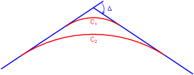 |
| Figure C-7 Different Arcs |
Both curves must accommodate a total direction change of Δ but since C1 is shorter it is sharper than C2.
Degree of curvature is a traditional way of indicating curve sharpness. There are two different definitions of degree of curvature: arc and chord.
Arc definition, Da, is the subtended angle for a 100.00 ft arc; Chord definition, Dc, is the subtended angle for a 100.00 ft chord, Figure C-8.
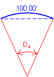 (a) Arc Definition |
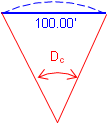 (b) Chord Definition |
| Figure C-8 Degree of Curvature |
|
Street and road alignments use the arc definition; chord definition is used for railroad alignments. For the remainder of this Chapter we will use the arc defintion and refer to it simply as D.
Degree of curvature is inversely proportional to radius: as D increases, R decreases, Figure C-9. The larger D is, the sharper the curve.
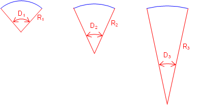 |
| Figure C-9 D and R Relationship |
Note the importance of 100.00 in both Degree of Curvature versions. This goes back to a standard tape length and stationing interval. However, in the metric system there is no convenient base equivalent of 100.00 ft. While design criteria was traditionally expressed in terms of D, it is more common today to instead use R which works for both the English and metric systems.
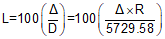
The relationship between D and R is expressed by Equation C-1.
 |
Equation C-1 |
b. Curve Components; Equations
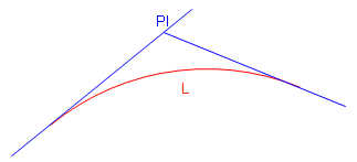
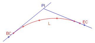
Figure C-10 shows a tangent circular arc with some basic components labeled.
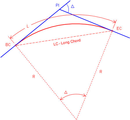 |
| Figure C-10 Basic Components of a Circular Arc |
|
PI |
Point of Instersection |
|
BC |
Begin Curve (aka: PC - Point of Curve; TC - Tangent to Curve) |
|
EC |
End Curve (aka: PT - Point of Tangent; CT - Curve to Tangent) |
|
Δ |
Defelction angle at PI; also the central angle of the arc |
|
R |
Arc radius |
|
L |
Arc Length |
|
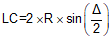
LC |
Long Chord length |
Figure C-11 includes additional curve components.
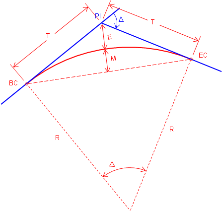 |
| Figure C-11 Additional Curve Components |
|
T |
Tangent distance |
|
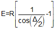
E |
External distance - from PI to midpoint of arc |
|
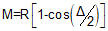
M |
Middle ordinate - distance between midpoints of arc and Long Chord |
Equations for the curve components are:
 |
Equation C-2 |
 |
Equation C-3 |
 |
Equation C-4 |
 |
Equation C-5 |
 |
Equation C-6 |
Although it may look like it in Figure C-11, E and M are not equal.
c. Stationing
As mentioned in Chapter A, an alignment is stationed at consistent intervals from its beginning through its end. On a finished desgin, the stationing should be along the tangents and the fitted curves.
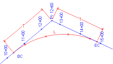
Traditionally, an alignment is stationed along the straight lines thru each PI, Figure C-12. Curve fitting comes later.
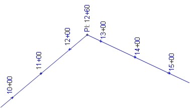 |
| Figure C-12 Stationing Along Tangents |
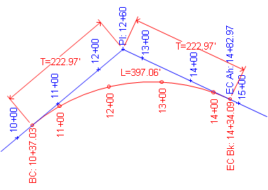
A circular curve is fit and staked. The stationing along the tangents between curve ends would be replaced by the curve stations, Figure C-13.
There are two ways to get from BC to EC:
(1) Up and down the tangents, T+T
(2) Along the curve, L
The distance along the curve is shorter than up and down the tangents: L < T+T
 |
| Figure C-13 Curve Inserted |
That means for a typical curve there are two stations for the EC:
One along the original tangents
One along the curve.
 |
|
Figure C-14 |
The EC station with respect to the original tangents is the EC Ahead. If we are standing on the EC and take a step ahead (up-station), we are on the tangent and its original stationing.
The EC station with respect to the curve is the EC Back. If we are standing on the EC and take a step back, we are on the curve and its stationing.
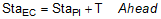
Chapter A mentioned that a station equation is used where one point has two stations. In this case we have a station equation at the EC: EC Sta Ahead = EC Sta Back. Figure C-15 is an example of a station equation indicator on a set of Wisconsin Dept of Trans highway plans.
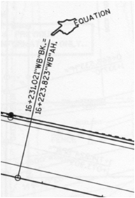 |
| Figure C-15 Station Equation Indicator |
A station equation represents a stationing discontinuity. We know the distance between two alignment points is their stationing difference. However if the points are on each side of an EC, the discontinuity must be taken into account. For example, the distance between stations 13+00 and 16+00 on the alignment shown in Figure C-14 is normally 300.00 ft but there are 48.88 ft "missing" at the EC. The 48.88 ft is the difference between the Ahead and Back stations: (14+82.97) - (14+34.09) = 48.88 ft. So the correct distance from 13+00 to 16+00 is 251.12 ft.
With software, it is possible to avoid station equations by waiting until the curves are fitted before stationing the entire alignment. With computer assisted designs, the PIs could be computed positions, Figure C-16.
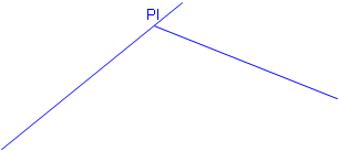 |
| Figure C-16 Computed Tangents and PVI |
A curve is then fit to the tangents, Figure C-17.
 |
| Figure C-17 A Curve is Fit |
Then the alignment is stationed from its beginning to its end through the curves, Figure C-18. That way there are no station equations.
 |
| Figure C-18 Stationing Through Curve |
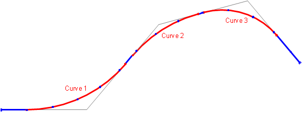
So this latter method is simpiler and the one that should be used, right? Well, it does have some advantages, but it also has disadvantages. What happens if the alignment design must be changed at some point later in the process?
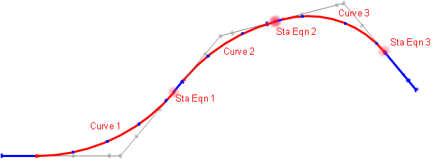
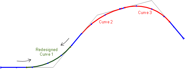
With traditional stationing, each curve has its own EC station equation. If one curve is altered, only its stationing is affected, no other stations on the alignment change, Figure C-19.
|
|
 (b) Limited Stationing Changes with Curve Modification |
| Figure C-19 Alignment with Station Equations |
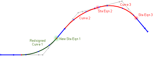
With continuous stationing, when a curve is altered it affects stations on it as well as all stations after it, Figure C-20.
 (a) Original Continuous Stationing |
 (b) Stationing Changes on and after Modified Curve |
| Figure C-20 Alignment with Continuous Stationing |
For example, if the redesigned curve is shorter, then all full (+00) station points after the curve increase. For example, 12+00 becomes 12+7.03, 13+00 becomes 13+07.03, etc. If the alignment is already staked then each stake could be renumbered or each could be each be moved back 7.03 feet. Hmm, odd stations or moving stakes.... Maybe station equations aren't so bad after all.
BC and EC stations are computed from the following formulae:
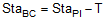 |
Equation C-7 |
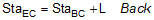 |
Equation C-8 |
 |
Equation C-9 |
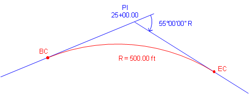
d. Example: Curve Components, Stationing
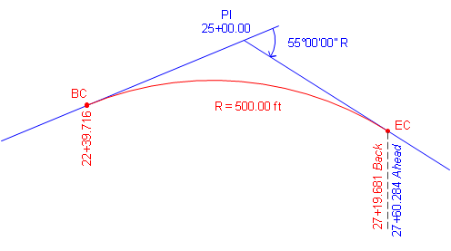
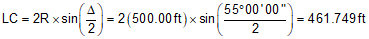
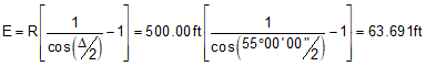
A PI is located at station 25+00.00. The deflection angle at the PI is 55°00'00" R. A 500.00 ft radius curve will be fit between the tangents.
Compute curve components and endpoint stations.
Start with a sketch:
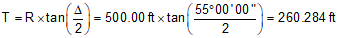
Use Equations C-2 through C-6 to compute curve components (carry an additional digit to minimize rounding errors):
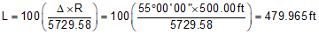

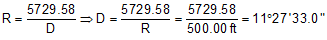
Compute degree of curvature using Equation C-1:
Use Equations C-7 through C-9 to compute endpoint stations: