E. Spirals
1. Concepts
Spirals were mentioned in the Basic Concepts section of Chapter C. Horizontal Curves. In this chapter, we will go into more detail.
Recall that a spiral arc, Figure E-1, has a constantly changing radius.
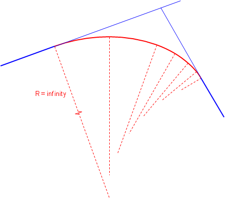 |
| Figure E-1 |
This characteristic has advantages in route applications, discussed in the next section, as well as presenting computational challenges. While a more complex geometric curve than a circular arc, a few reasonable assumptions can simplify its calculation.
2. Applications
a. Direction transition
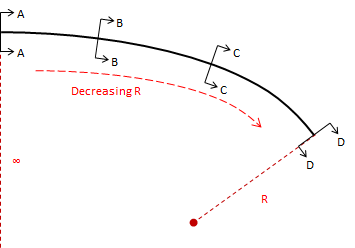
Because curvature is introduced progressively, the driver gradually changes the steering wheel angle allowing a more natural direction transition.
 |
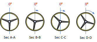 |
| Figure E-2 Steering wheel angle along a spiral |
b. Force balancing
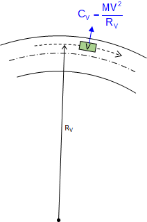
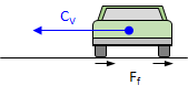
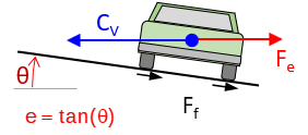
A vehicle traveling a curved path at constant velocity is subject to a centrifugal force, CV, pushing it (and its occupants) to the outside of the curve, Figure E-3(a). If the pavement cross-slope is flat, only the friction between the tires and road surface prevents the vehicle from sliding off the curve, Figure E-3(b). In low friction situations (rain, snow, etc), sliding will occur at lower speeds. Banking the pavement cross-slope into the curve, Figure E-3(c), allows part of the vehicle weight to work with friction to offset the centrifugal force. This banking is called superelevation, e.
 |
 |
| (b) Flat pavement cross-slope | |
 |
|
| (a) Centrifugal force | (c) Superelevation added |
| Figure E-3 Balancing forces |
|
At the right combination of vehicle speed and superelevation, friction does not come into play - the pavement can be ice covered and the vehicle will not slide off the curve.
With a circular curve, centrifugal force is theoretically introduced immediately upon curve entry. This doesn't typically happen because it takes the driver some distance to change the steering wheel angle from straight ahead to full-turn. Deciding where to begin rotating the cross-slope from flat and how quickly to reach full superelevation requires some compromises.
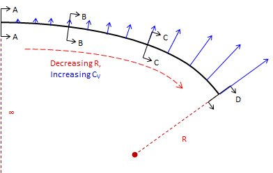
A spiral helps because its decreasing radius increases centrifugal force gradually, Figure E-4, so superelevation can be introduced at a corresponding rate keeping forces balanced.
 |
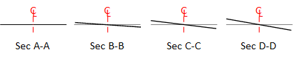 |
| Figure E-4 Cross-section along a spiral |
It is primarily because of this force balancing characteristic that spirals are used in high-speed railroad alignments. More on that in the yet-to-be-developed Superelevation chapter.
c. Design flexibility
Combining spirals with (or without) intermediate circular arcs allows greater design flexibility particularly in limited spaces and where large directional changes are involved. Consider the two alignment segments in Figure E-5(a) which are to be connected via a cloverleaf interchange. Traveling North to West, the directional change is 270° degrees. Figure E-5(b) shows three alternative curve systems to connect the two alignments. This interchange type is used extensively in high speed situations where the driver must decelerate, negotiate a large direction change, then accelerate to match traffic. It should be a smooth and surprise-free driver experience.
 |
 |
| (a) Intersecting alignments | (b) Alternative curve systems |
| Figure E-5 Cloverleaf interchange | |
The green system is a single tangent circular arc. Even though it is a relatively sharp curve, it takes up the most space (to take up less space, it would need to be even sharper). Its primary shortcomings are the tangent-curve-tangent transitions and centrifugal force condition requiring a lower speed and higher superelevation.
The red system is a five-center compound curve using consecutive curves of varying radii. The concept behind this application was discussed in Chapter D. Multi-Center Horizontal Curves. While better than the single curve and taking up less space, it can still be problematic at the curve-curve transitions since the forces can change substantially unless speeds are reduced.
The blue system is a spiraled horizontal curve: an entrance spiral into a circular arc into an exit spiral. In this example, this is a symmetric system with entrance and exit spirals mirror images of each other, although that needn't be the case. Not only does this curve system provide the smoothest speed and direction changes, it is the most comfortable and takes up the least space.
3. Nomenclature & Parts
A single figure showing a spiraled horizontal curve with all its nomenclature, parts, and points labeled can be confusing. To make things a little more clear, we will use a series of figures emphasizing and explaining different attributes. Although ours will be a symmetric curve system, the same principles apply to differing entrance and exit spirals, as long as sufficient basic information is known.
Let's start with two tangents and a circular curve of radius Rc and length L connecting them, Figure E-6.
 |
|
Figure E-6
Simple curve between tangents |
To make room for spirals inclusion requires pushing the circular arc in from the tangents and shortening its length. Adding two spirals, each Ls long, reduces the circular arc length to Lc. This results in the TS-SC-CS-ST curve system, Figure E-7. The OBC and OEC are offset positions of the BC and EC. Radial lines from the OBC and OEC to the arc's center of curvature are parallel with perpendicular lines at the TS and ST respectively.
 |
Ls: Spiral length Lc: Reduced arc length Rs: Spiral radius (varies) Rc: Circular arc radius TS: Tangent to Spiral SC: Spiral to Curve CS: Curve to Spiral ST: Spiral to Tangent OBC: Offset BC OEC: Offset EC |
| Figure E-7 Spiraled horizontal curve |
|
The radius of the entrance spiral, Rs, decreases uniformly from infinity at the TS to the circular arc radius, Rc, at the SC. The radius of the exit spiral increases uniformly from the arc radius at the CS to infinity at the ST.
The entrance spiral's degree of curvature, Ds, varies from 0°00'00" at the TS to the circular arc's, Dc, at the SC. Because it changes uniformly over the spiral's length, its rate is Equation E-1:
| Equation E-1 | k: Spiral's Degree of Curvature rate change Dc: Circular arc D Ls: Spiral length |
Although reversed, the exit spiral in a symmetric system has the same k.
Figure E-8 shows the central angles (Δ) for the spirals and circular arc.
 |
Δs: Spiral Central Angle Δc: Circular Curve Central Angle |
| Figure E-8 Central Angles |
|
Because the radial lines at the TS and OBC are parallel, the central angle of the entrance spiral is the same as the central arc angle from the OBC to the SC. The same is true for the exit spiral. The spiral angle is determined from Equation E-2.
| Equation E-2 |
The original circular arc's central angle is reduced by the spirals', Equation E-3.
| Equation E-3 | Δc: Reduced arc central angle Δ: Total central angle Δs: Spiral central angle |
And its shortened length is determined from Equation E-4 (modified from Chapter C. Horizontal Curves).
| Equation E-4 |
Location of the TS from the PI along with tangent distances and offsets from the TS to the OBC and SC are shown in Figure E-9.
 |
 |
| (a) | (b) |
|
LCs: Spiral long chord
A: Spiral deflection angle Ts: Spiral tangent |
Xo: Tangent distance to OBC
o: Tangent offset to OBC X: Tangent distance to SC Y: Tangent offset to SC |
| Figure E-9 Tangent Distances |
|
The distances and offsets are computed using Equations E-5 through E-10
| Equation E-5 | |
| Equation E-6 | |
| Equation E-7 | |
| Equation E-8 | |
| Equation E-9 | |
| Equation E-10 |
Because spirals are short and very flat, arc distances are often used to approximate chord distances. The is the case with Equations E-5 through E-7: the spiral length, Ls, is used for the spiral chord, LCs. In most cases, this assumption will be fine, however, we'll discuss a more exact, though more complex, spiral computing method also.
4. Stationing
Referring to Figure E-7, curve endpoint stations are determined using Equations E-11 through E-15.
| Equation E-11 | |
| Equation E-12 | |
| Equation E-13 | |
| Equation E-14 | |
| Equation E-15 |
As with a regular horizontal curve, a station equation exists at the point where the curve system exits onto the tangent at the ST.
5. Deflection Angle Method
The traditional method of staking a spiral is by measuring a deflection angles at the TS and chords between curve points. In Figure E-10, the process to lay out the first two points after the TS are:
- Instrument at TS, sighting PI.
- To stake point i
- Rotate to deflection angle of i, ai.
- Measure distance LTSI-i
- Stake point j
- Rotate to deflection angle of j, aj.
- Measure distance Li-j
The arc distances between the points (ie, Staj - Stai) are used as chords. While this does introduce some error, because of the spiral's geometry, the error is relatively small.
 |
| Figure E-10 Deflection Angle Method |
General calculations are based on these spiral properties for any point referenced to the flat end:
- Radius is inversely proportional to distance along the spiral.
- Spiral angle is proportional to the square of the distance
- Deflection angle is closely proportional to the square of the distance
- Tangent offset is closely proportional to the cube of the distance.
 |
| Figure E-11 Deflection Angle Geometry |
For any spiral point i:
| Equation E-16 | Arc distance | |
| Equation E-17 | Spiral radius | |
| Equation E-18 | Spiral angle, radians | |
| Equation E-19 | Spiral angle, degrees | |
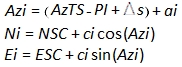
| Equation E-20 | Deflection angle, degrees |
Although not needed for the traditional deflection angle method, the tangent distance and offset to a curve point, Figure E-12, can be computed using Equations E-21 and E-22.
 |
|
||||
| Figure E-12 Tangent Distance and Offset |
Tangent distances (xi) and offsets (yi) can be used to compute radial chords from the TS to the respective curve point, Figure E-13 and Equation E-23.
 |
| Figure E-13
Radial Chord
|
| Equation E-23 |
As with the point-to-point condition, generally the arc distances can be used as radial chord distances. We see this shortly in an example.
6. Five- or ten-chord spiral
It is common to compute (and stake) a spiral in equal intervals rather than full- or half-stations. Depending on spiral length and arc degree of curvature, the spiral is computed in either five or ten equal intervals. For example, a 200 foot five-chord spiral would be computed at a 40 foot interval.
Although this results in spiral points with odd stations, its advantage is a single set of calculations for the entrance and exit spirals. Because the deflection angle method is computed from a spiral's flat end, TS for the entrance and ST for the exit, the same equal interval computations can be used for both. We'll see this in the following example.
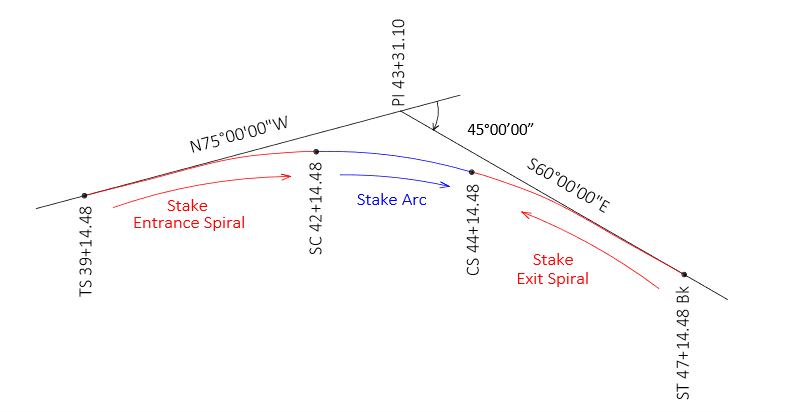
7. Example Spiraled Horizontal Curve Computation
a. Set up
A N75°00'00"E tangent intersects a S60°00'00"E tangent at station 43+31.10. A circular arc with a 9°00'00 degree of curvature will be used together with 300.00 ft entrance and exit spirals.
Compute radial stake out notes using 5-chord spirals and arc half stations.

b. Spiral components
c. Circular curve components
d. Stationing
| StaPI | 43+31.10 | StaPI | 43+31.10 | |||
| -Ts | 4+16.62 | +Ts | 4+16.62 | |||
| StaTS | 39+14.48 | StaST | 47+47.72 | Ahead | ||
| +Ls | 3+00.00 | |||||
| StaSC | 42+14.48 | |||||
| +Lc | 2+00.00 | |||||
| StaCS | 44+14.48 | |||||
| +Ls | 3+00.00 | |||||
| StaST | 47+14.48 | Back |
e. Five-chord spiral
Length of each chord:
![]()
Deflection angle equation
![]()
Set up the curve table and solve ai for each curve point. Indicate appropriate math checks.
| Chord Num | li, ft | ai | ||
| 1 | 60.00 | 0°10'48" | ||
| 2 | 120.00 | 0°43'12" | ||
| 3 | 180.00 | 1°37'12" | ||
| 4 | 240.00 | 2°52'48" | ||
| 5 | 300.00 | = Ls | 4°30'00" | = Δs/3 |
Set up and solve Equations E-21 through E-23 for radial chords:
| Chord Num | li, ft | ai | xi, ft | yi, ft | ci, ft | ||
| 1 | 60.00 | 0°10'48" | 60.00 | 0.00 | 60.00 | ||
| 2 | 120.00 | 0°43'12" | 119.99 | 1.51 | 120.00 | ||
| 3 | 180.00 | 1°37'12" | 179.93 | 5.09 | 180.00 | ||
| 4 | 240.00 | 2°52'48" | 239.71 | 12.06 | 240.00 | ||
| 5 | 300.00 | 4°30'00" | 299.07 | = Y | 23.56 | = X | 300.00 |
Notice that the radial chord to each point is the same as its spiral distance. Because the spiral is short and flat, spiral arc and radial chord distances are (essentially) the same. That simplifies spiral computations and staking considerably: use arc distance as radial chord for each point.
f. Circular arc deflections
Set up Equations C-12 through C-15 from Chapter C. Horizontal Curves:
The curve table, with appropriate math checks, is:
| Stai | li, ft | defl angi | ci, ft | ||||
| CS | 44+14.48 | 200.00 | = Lc | 9°00'00" | = Δc/2 | 199.18 | = LC |
| 44+00 | 185.52 | 8°20'54" | 184.86 | ||||
| 43+50 | 135.52 | 6°05'54" | 135.26 | ||||
| 43+00 | 85.52 | 3°50'54" | 85.46 | ||||
| 42+50 | 35.52 | 1°35'54" | 35.52 | ||||
| SC | 42+14.48 | 0.00 | 0°00'00" | 0.00 |
g. Stake out notes
Now to assemble the information into a single set of notes:
| Station | Defl Ang | Radial chord, ft | |
| Exit Spiral Occupy ST, Backsight CS |
|||
| ST | 47+14.48 | 0°00'00" | 0.00 |
| 46+54.48 | 0°10'48" | 60.00 | |
| 45+94.48 | 0°43'12" | 120.00 | |
| 45+34.48 | 1°37'12" | 180.00 | |
| 44+74.48 | 2°52'48" | 240.00 | |
| CS | 44+14.48 | 4°30'00" | 300.00 |
| Circular Arc Occupy SC, Backsight CS |
|||
| CS | 44+18.48 | 9°00'00" | 199.18 |
| 44+00 | 8°20'54" | 184.86 | |
| 43+50 | 6°05'54" | 135.26 | |
| 43+00 | 3°50'54" | 85.26 | |
| 42+50 | 1°35'54" | 35.52 | |
| SC | 42+14.48 | 0°00'00 | 0.00 |
| Entrance Spiral Occupy TS,Bbacksight SC |
|||
| SC | 42+14.48 | 4°30'00" | 300.00 |
| 41+54.48 | 2°52'48" | 240.00 | |
| 40+94.48 | 1°37'12" | 180.00 | |
| 40+34.48 | 0°43'12" | 120.00 | |
| 39+74.48 | 0°10'48" | 60.00 | |
| TS | 39+14.48 | 0°00'00" | 0.00 |
 |
|
Figure E-14
Staking a Spiraled Horizontal Curve
|
8. Staking a Spiraled Horizontal Curve
a. Establish TS and ST
Set TS and ST points at distance Ts from PI along each tangent.
b. Stake entrance spiral
Set instrument at TS.
Backsight PI with 0°00'00" on horizontal circle.
Radially stake each spiral point through the SC.
c. Stake circular arc
Because it is offset from the tangents, the arc can't be staked from a BS using the PI as a backsight. Instead, once the entrance spiral has been staked, the circular arc must be staked from the SC.
At the flat end of the spiral, the deflection angle is (Δs)/3; at the other end it is (2Δs)/3, Figure E-15.
 |
| Figure E-15 Spiral Total Deflection Angles |
To correctly orient an instrument at the SC, the surveyor would, Figure E-16:
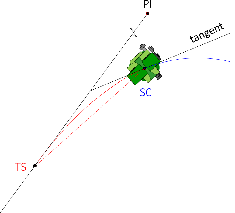 |
Set up on SC. Backsight the TS with -(2Δs)/3 on the horizontal circle. |
 |
Rotate to 0°00'00". Instrument in now tangent to the spiral and circular arc. |
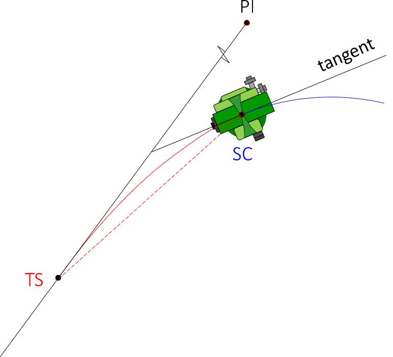 |
Reverse telescope about the horizontal axis. Instrument is sighting where the arc's PI would be. Stake the curve to the CS using the deflection angle information |
| Figure E-16 Staking the Circular Arc |
|
b. Stake exit spiral
Set instrument at ST.
Backsight PI with 0°00'00" on horizontal circle.
Radially stake each spiral point through the CS.
The CS serves as a closure check since it was placed when the arc was staked.
9. Power Series Method
a. Equations
A more accurate way to compute spiral points is using infinite power series, Equations E-24 and E-25.
| Equation E-24 | |
| Equation E-25 |
δi in Equations E-24 and E-25 is in radians; it is computed with Equation E-18.
Although both equations have an infinite number of terms, each term is substantially smaller so only the first three need be used.
Radial chords are computed using Equation E-23 and deflection angles using Equation E-26.
 |
Equation E-26 |
b. Example
Using the spiral of the previous example, set up and solve the spiral curve table.
![]()
| Chord Num | li | δi, radians | xi, ft | yi, ft | ci, ft | ai |
| 1 | 60.00 | 0.009425 | 60.00 | 0.19 | 60.00 | 0°10'48" |
| 2 | 120.00 | 0.037699 | 119.98 | 1.51 | 119.98 | 0°43'12" |
| 3 | 180.00 | 0.084823 | 198.87 | 5.09 | 179.87 | 1°37'12" |
| 4 | 240.00 | 0.150796 | 239.46 | 12.04 | 239.46 | 2°52'46" |
| 5 | 300.00 | 0.235619 | 298.34 | 23.47 | 298.34 | 4°29'52" |
Compare this curve table to the first table in Section 7e. The results of this "more exact" calculations are basically the same as those based on approximations.
Should a much longer spiral or one with a great radii difference be used, the approximations may be might introduce measurable error in which case the power series equations should be used.
10. Spirals and Coordinates
As with most surveying stake out operations, having point coordinates makes for more flexible field operation.
Starting with directions of the incoming and outgoing tangents along with the PI coordinates, the process to compute point coordinates are:
a.TS and ST coordinates, Figure E-17
 |
| Figure E-17 TS and ST Coordinates |
These are computed using Equations E-27 through E-31.
 |
Equations E-27 through E-29 |
 |
Equations E-30 and E-31 |
b. Spiral point coordinates, Figure E-17
 |
| Figure E-17
Spiral Coordinates
|
Using the deflection angle notes, spiral point coordinates can be computed using Equations E-32 through E-37. Right deflection angles are positive, left are negative.
| Entrance spiral | |
 |
Equations E-32 through E-34 |
| Exit spiral | |
 |
Equations E-35 through E-37 |
c. Arc point coordinates, Figure E-18
 |
| Figure E-18 Arc Coordinates |
Arc points are computed using equations E-38 through E-40. Right deflection angles are positive, left are negative.
 |
Equation E-38 through E-40 |
Math check? The coordinates of the CS computed from the SC should match those computed from the ST.
11. Spreadsheet
An Excel spreadsheet to perform basic spiral computations can be downloaded here. It uses Visual Basic for Applications script so Excel must have macros enabled when loading the sheet.
12. Summary
Although more geometrically complex than circular arcs, spirals are relatively easy to compute using approximate relationships. The argument against their use due to computation complexity really isn't valid as shown by the example.
However, despite their transportation applications advantages, spiral use is limited primarily to railroads. Trains have a mechanical connection between wheel flanges and rails, in essence, infinite friction. Because the train's wheels cannot slip across the rails as can tires on pavement, lateral force is directly imparted to the rails as the train enters and travels around a curve. If a simple curve is used, then maximum centrifugal force is instantaneously introduced at the BC since the train must follow the tracks. A spiral's changing radius allows the centrifugal force to gradually increase (entrance) then decrease (exit), balancing the forces. Running a train over an simple horizontal curve over time will eventually shift the rail alignment into a spiraled configuration because of the forces.
In high speed highway designs, horizontal circular curves are typically long and flat, making for smooth tangent-curve-tangent transitions, minimal centrifugal force, and lower superelevation rates. Spirals aren't needed in these situations. Spirals can be used beneficially in case of large direction changes over limited areas, such as interchanges.
Spiral use is up to the designer but as shown in this Chapter, they are not difficult to understand and their computation not much more arduous.