I. Curve Fitting
A. Introduction
Curve fitting is the process of determining the mathematical relationshp between data series in a 2D set. The phrase "curve fitting" comes from a traditional graphic solution: the data is plotted, a line or smooth curve is drawn through the data points, and an equation computed by measuring on or interpreting from the graph. If the data contains measurements, there will be random errors so a perfect fit is not possible. The line or curve will not pass through all the points so a visual best-fit curve is drawn.
With enough data points least squares can be used to numerially determine a best-fit equation.
B. Types of variables
Two-dimensional data is based on two variables: an independent variable and a dependent one. The dependent variable's value is based on the value of the independent one. The equation relating the variables indicates what happens to the dependent variable as the independent one changes.
With measurements, the independent variable values indicate where they are made, the dependent variable values are the measurements.
When plotting data, the independent variable is on the x-axis while the dependent is on the y-axis, Figure I-1.
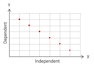 |
| Figure I-1 Plotting Data |
C. Theoretical vs Empirical
The independent and dependent variable relationship can be either theoretical or empirical.
1. Theoretical
A theoretical relationship is based strictly on a mathematical equation; there are no observed or measured data. There is an exact relationship between the two so there is no error.
A basic example in surveing is a proposed grade line in an alignment design. A +3.0% grade begins at station 10+00 with elevation 800.0.and ends at station 13+00. For every 100 ft horizontally, elevation changes 3.0 ft vertically. Expressed as an equation:
| Elev = 800.0+d(g) | ||
| g: 0.03 | ||
| d: distance from sta 10+00, in ft | ||
We select a station and compute its elevation; elevation is the dependent variable.
Set up a table for elevations at full stations, Table I-1
| Table I-1 Grade Elevations |
|
| Station | Elevation |
| 10+00 | 800.0 |
| 11+00 | 803.0 |
| 12+00 | 806.0 |
| 13+00 | 809.0 |
Although the table shows only four data pairs, because theirs is an exact relationship, we can add as many as we like: 801.5 ft at 10+50, 804.5 at 11+50, etc.
The table is one way to look at the data, plotting it is another way to visualize it. Using the same scale for both axes, Figure I-2, results in a very flat plot that is difficult to interpret. That's because elevation changes only 9.0 ft while stationing changes 300 ft, a 1:33.33 ratio.
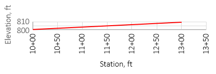 |
| Figure I-2 Grade; Same X and Y scales |
Increasing the elevation scale exaggerates the plot vertically and makes the data grade line more apparent. Figure I-3 uses a vertical exaggeration of 10:
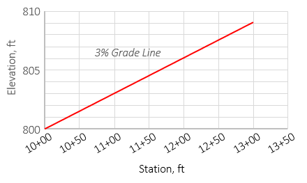 |
| Figure I-3 Grade; Vertical exaggeration 10 |
Because a theoretical plot is based on a mathematical equation, there are infinite data points. When the graph is drawn, only the line or curve is shown, not individual data points.
2. Empirical
Empirical data is based on measurement or observation. The dependent variable is measured at a specific independent values. Being measured, the dependent values are is subject to errors; the independent ones are considered error-free.
Let's use another surveying example. A profile level is run along a section of center line on existing terrain. The results are in Table I-2.
| Table I-2 Profile Level |
|
| Station | Elevation |
| 22+00 | 1250.2 |
| 23+00 | 1248.7 |
| 24+00 | 1245.5 |
| 25+00 | 1243.8 |
Plotting the data, using a vertical exaggeration of 4, Figure I-4:
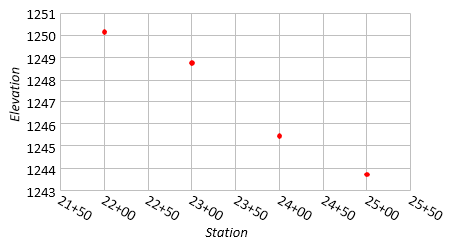 |
| Figure I-4 Profile Elevations |
It looks like a straight line will fit ... but will it? Since two points define a straight line, we can construct a whole bunch of grade lines, Figure I-5.
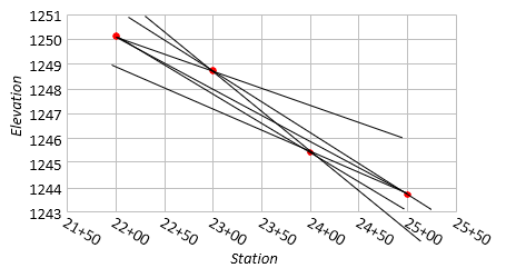 |
| Figure I-5 Multiple Straight Lines |
Any single line fits two points perfectly, but misses the other two, sometimes by quite a lot.
Draw a best-fit line which may or may not go through individual data points but meets some specific criteria, Figure I-6
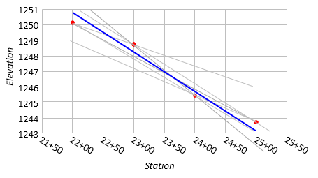 |
| Figure I-6 Best-fit Straight Line |
Because this is a linear relationship, a best-fit line represents acceptable compromises but must still be straight.
D. Fitting a Straight Line
1. Equation
The equation of a straight , Figure I-7,line is:
| y = mx+b | Equation I-1 | |||
| m is the line slope b is the y intercept |
||||
 |
| Figure I-7 Straight Line Geometry |
Slope, m, is rise/run. It is also the tangent of the angle from the x-axis to the line; m = tan(θ).
2. Residuals
Empirical data doesn't exactly fit a straight line because:
- the objects measured may not have a linear relationship
- the measurements have random errors
A best-fit straight line is one which minimizes the sum of the squares of the residuals, Figure I-8.
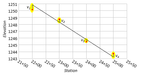 |
| Figure I-8 Profile Residuals |
The residual is the difference between the theoretical and empirical values at an independent variable, Equation I-2
| vi = Yt - Ye | Equation I-2 | ||
| Yt - theoretical value | |||
| Ye - empirical value | |||
3. Least Squares
The best-fit line minimizes the sum of the residuals squared, Equation I-3
| Σ(vi)2= minimum | Equation I-3 |
There are two least squares solution methods for a straight line: Linear regression and Observation equations. Each has its particular advantage(s) and disadvantage(s).
a. Linear Regression
Linear regression can be done manually or using a built-in function on most scientific calculators. It is a standard function in most spreadsheet software and included in their graphic options (aka, trendline).
The line slope, m, is determined using Equation I-4:
 |
Equation I-4 |
and intercept, b, from Equation I-5:
| Equation I-5 |
The correlation coefficient, r, indicates how well the data fits a straight line.
 |
Equation I-6 |
| Equation I-7a | |
| Equation I-7b |
The coefficient varies between -1 (negatively sloped line) and +1 (positively sloped line); the closer to -1 or +1, the better the data fits a straight line.
b. Observation Equations
An observation equation is written for each coordinate pair. Then one of two ways can be used to reach the solution:
1. Direct minimization: This is covered in Chapter C.
2. Matrix method: This is covered in Chapter D.
Direct minimization is the most arduous method requiring a considerable amount of computations to perform manually. Anything over four coordinate pairs increase computations substantially. The matrix method is more efficient and easier perform, even manually without benefit of software.
4. Application Example
Let's determine the best-fit line for the measured profile data of Table 2.
a. Linear regression
Organizing the data in an extended table simplifies computations, particularly since some of the terms are so large.
X is Station, Y is Elevation.
| X, ft |
Y, ft |
X2 |
vx | vy | (vx)(vy) | vx2 |
vy2 |
|
| 2200 | 1250.2 | 4,840,000 | 2195 | 1225.20 | 2,689,319.49 | 4,818,025 | 1,501,121.2 | |
| 2300 | 1248.7 | 5,290,000 | 2295 | 1223.70 | 2,808,397.24 | 5,267,025 | 1,497,447.8 | |
| 2400 | 1245.5 | 5,760,000 | 2395 | 1220.50 | 2,923,103.49 | 5,736,025 | 1,489,626.4 | |
| 2500 | 1243.8 | 6,250,000 | 2495 | 1218.80 | 3,040,912.24 | 6,225,025 | 1,485,479.5 | |
| sums |
9400 | 4988.2 |
22,140,000 | 9380 | 4888.20 | 11,461,732.46 | 22,046,100 | 5,973,674.9 |
Substituting terms in the linear regression equations:

The best-fit equation is: Elev = -0.0224(Station) + 1299.69
The correlation coefficient is -0.99 which is a pretty good fit.
Because Stations are used for x values, the slope, m, is the grade expressed as a ratio: grade = -0.0224 ft/ft = -2.24%
The simplicity of the table belies all the computations needed to construct it. The primary disadvantage of Liner Regression is the amount of calculations if done manually. It's quick, however, if using built-in calculator or spreadsheet functions.
b. Matrix Method
An observation equation is written for each data pair, using Equaton I-1, with a residual included on each dependent variable:

In matrix notation, the observation equations are [K] + [V] = [C] x [U].
The matrices are:

The matrix algorithm [U] = [Q] x [CTK] is solved to determine m and b.
Instead of the complete solution process step-by-step, intermediate products are shown:

Since the [CTC] matrix is only 2x2, it can be quickly inverted using the determinant method.
The matrix algorithm results are m = -0.0224 and b = 1299.69 just like Linear Regression's results.
Surprise.
While there is no direct equivalent to the correlation coefficient, the uncertainties for m and b can be determined.
Using the equations from Chapter D Section 3:

E. Interpolation, Extrapolation
1. Purpose
One of the reasons we fit a line or equation to data is to allow determination of one variable based on fixing the other variable's value. For example, Figure I-9 is a graph of a steel tape's length at differnt pull amounts.
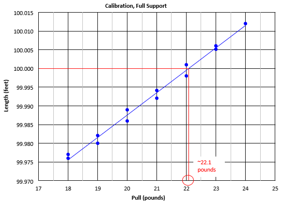 |
| Figure I-9 Tape Pull Clibration |
As pull was changed, the tape length was measured against a calibrartion line; length is dependent on pull.
The equation of a best-fit line determined by Linear Regression is L = 0.0059P+99.869.
2. Interoplation
How much pull should be applied to achive 100.000 ft? We can determine the pull by either scaling it from the graph (22.1, shown in red) or by solving the equation:
100.000 = 0.0059P+99.869 arrange to solve for P: P = (100.000-99.869)/0.0059 = 22.2 lbs.
This is called interpolation: using the data to predict one variable value from the other.
Interpolation is done within the data range. When collecting measurements, we try to bracket the range that we may later want to determine.
For example, we calibrate a tape to determine the conditions necessary for its length to be 100.000 ft. We started with a pull that yielded a tape length less than 100.000 ft then progressively increased pull until the length exceeded 100.000 ft. Then we progressicvely decreased pull until the length was less than 100.000 ft. We have enough data on both sides of 100.000 ft to reliably determine the pull needed to achieve it.
3. Extrapolation
Using the same data in Figure I-9, what will be the tape length when 25 pounds of pull are applied?
We can't determine it directly from the graph because it doesn't go out far enough. We could extend it the graph, but that's a bit cumbersome. Or we can use the equation:
L = 0.0059P+99.869 = 0.0059(25)+99.869 = 100.016 ft
This is extrapolation: predicting one variable value from the other outside the data range.
Extrapolations should be limited to values very close to the data range. The line fit is based on the behavior within the data range. We don't know what happens outside that range. Just because we can determine an equation doesn't mean it's a good predictor outside the range.
For example, how much pull would be needed to strech tape to 105.000 ft? From the equation, it would be:
P = (105.000-99.869)/0.0059 = 870 lbs
Not only is 870 lbs an unreasonable amount to attempt, the tape itself would fail before that. At some point it reaches its plasticity limit and won't return to its original length; keep going and it eventually will fail by breaking. We can't determine either of those based this data set because it is below the failure threshhold.
We generally leave extrapolation to economists, politicians, and weather forecasters.
F. Curved Lines
1. General
Not all data relationships are linear. The graph in Figure I-10 are the results of an aerial camera calibration for radial lens distortion. The distortion is caused by lens material and surface curvature. Its effect is measured on the image plane at radial intervals from the principal point.
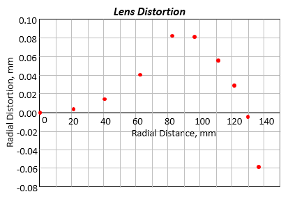 |
| Figure I-10 Lens Distortion Data |
It's obvious the data doesn't fall on a straight line, but it doesn't follow a simple curve either. So how do we fit a curve to nonlinear data? Linear regression can't be used to fit a curve because, well, the curve isn't straight.
Actually, linear regression can be used in some cases if the logarithm of the dependent variable or logarithms of both variables are used. But those are exceptions to the rule, we want a universal method.
Let's examine a few surveying applications.
2. Vertical Curve
Table I-3 lists some elevations at particular stations through which it is desired to run a vertical alignment curve.
| Table I-3 | |
| Station | Elevation |
| 11+00 | 848.8 |
| 12+00 | 850.7 |
| 13+00 | 851.1 |
| 14+00 | 850.3 |
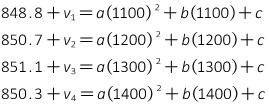
A verical curve is part of a parabola whch is a second-degree polynomial. That means its equation includes a squared independent variable term, Equation I-8.
| y = ax2+bx+c | Equation I-8 |
Where two points are needed to define a straight line, three points are needed for a second-degree polynomial. Why three points? Because there are three unknown coefficients: a, b, and c. More than three allows a least squares solution; each point beyond three is a redundancy.
We don't have to stop there. We can get much more complex: a nth degree polynomial needs n+1 points to fix and >n+1 points for a least squares solution. However, we'll stick to second degree polynomials for now since they cover the bulk of complex survey curves.
The data in Table I-3 is plotted in Figure I-11 along with a best-fit parabolic curve.
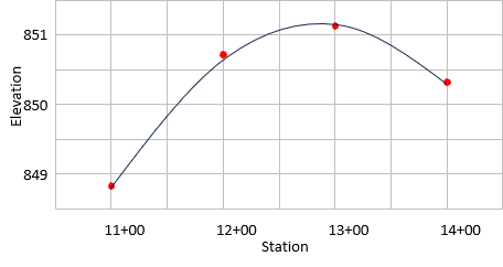 |
| Figure I-11 Best-Fit Vertical Curve |
To determine the curve equation, Equation I-8 is used to develop the observation equations, with the residual term on the Y (Elevation) value.
The matrices are:

Now we just solve the matrix algorithm [U] =[Q] x [CTK]
Intermediate products:

Coefficients:

The equation is:
![]()
Notice that many intermediate matrix elements are either extremely large or small. That's not an issue using software to manipulate the matrices, but manual calculations can lead to errors. One way to lessen potential errors is to divide the stations by 100, reducing their size. The observation equations coefficient matrix becomes:

The [Q] matrix:

And the coefficients:

Compare the these coefficients with the solution using the full station expression:
a increases by 10,000 = 1002 which corresponds to a2
b increase by 100 which corresponds to b
c is the same
That means the equation can be written as
![]()
or
![]()
where S = Sta/100
3. Horizontal Curve
Probably the most prevalent curve that surveyors deal with are horizontal which use circular arc sections. These are also second degree polynomials but unlike a parabola, they have constant radii. Another difference is there is really no dependent-independent variable distinction. The data points for a horizontal curve are coordinates (X/Y or N/E), neither direction superior to the other.
Being a second-degree polynomial, three points are needed to define it.
Equation I-9 is used to solve the arc if one of the points is the radius point, O, Figure I-12.
| Equation I-9 | |||||
|
where: Np, Ep - coordinates of a point on the arc |
|||||
 |
|||||
| Figure I-12 Including radius point |
|||||
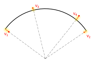
Equations I-10 and I-11 are used to solve the arc if all three points are on the arc, Figure I-13.
| Equation I-10 | |||
 |
Equation I-11 | ||
 |
|||
| Figure I-11 Only arc points |
|||
Four points allows a least squares solution.
Example
Determine the radius for the arc in Figure I-12 using the coordinates of the four arc points in Table I-4.
 |
| Figure I-12 Least Squares Arc Fitting |
| Table I-4 | ||
| Point |
E | N |
| 1 | 117.68 | 806.74 |
| 2 | 690.37 | 795.29 |
| 3 | 316.93 | 940.81 |
| 4 | 618.34 | 873.55 |
Use the coordinates and Equation I-10 to set up the observation equations. Include a residual on the constant term.

Create the initial matrices

Intermediate matrix

Solution matrix

Substitute the solution coefficients into the arc equation.
![]()
Determine the curve radius

Residuals
The observation equation form of equations I-9 and I-10 are:
| |
Equation I-12 |
| |
Equation I-13 |
In Equation I-12 the residual is on the radius which is a function of the coordinates.
In Equation I-13 the residual is on the arc point coordinates.
This makes the residuals perpendicular to the arc (radial), Figure I-13, since there is no dependent-independent variable condition.
 |
| Figure I-13 Curve Fit Residuals |