D. Fitting a Straight Line
1. Equation
The equation of a straight , Figure I-7,line is:
| y = mx+b | Equation I-1 | |||
| m is the line slope b is the y intercept |
||||
 |
| Figure I-7 Straight Line Geometry |
Slope, m, is rise/run. It is also the tangent of the angle from the x-axis to the line; m = tan(θ).
2. Residuals
Empirical data doesn't exactly fit a straight line because:
- the objects measured may not have a linear relationship
- the measurements have random errors
A best-fit straight line is one which minimizes the sum of the squares of the residuals, Figure I-8.
 |
| Figure I-8 Profile Residuals |
The residual is the difference between the theoretical and empirical values at an independent variable, Equation I-2
| vi = Yt - Ye | Equation I-2 | ||
| Yt - theoretical value | |||
| Ye - empirical value | |||
3. Least Squares
The best-fit line minimizes the sum of the residuals squared, Equation I-3
| Σ(vi)2= minimum | Equation I-3 |
There are two least squares solution methods for a straight line: Linear regression and Observation equations. Each has its particular advantage(s) and disadvantage(s).
a. Linear Regression
Linear regression can be done manually or using a built-in function on most scientific calculators. It is a standard function in most spreadsheet software and included in their graphic options (aka, trendline).
The line slope, m, is determined using Equation I-4:
 |
Equation I-4 |
and intercept, b, from Equation I-5:
| Equation I-5 |
The correlation coefficient, r, indicates how well the data fits a straight line.
 |
Equation I-6 |
| Equation I-7a | |
| Equation I-7b |
The coefficient varies between -1 (negatively sloped line) and +1 (positively sloped line); the closer to -1 or +1, the better the data fits a straight line.
b. Observation Equations
An observation equation is written for each coordinate pair. Then one of two ways can be used to reach the solution:
1. Direct minimization: This is covered in Chapter C.
2. Matrix method: This is covered in Chapter D.
Direct minimization is the most arduous method requiring a considerable amount of computations to perform manually. Anything over four coordinate pairs increase computations substantially. The matrix method is more efficient and easier perform, even manually without benefit of software.
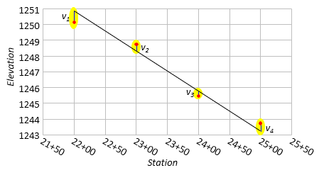
4. Application Example
Let's determine the best-fit line for the measured profile data of Table 2.
a. Linear regression
Organizing the data in an extended table simplifies computations, particularly since some of the terms are so large.
X is Station, Y is Elevation.
| X, ft |
Y, ft |
X2 |
vx | vy | (vx)(vy) | vx2 |
vy2 |
|
| 2200 | 1250.2 | 4,840,000 | 2195 | 1225.20 | 2,689,319.49 | 4,818,025 | 1,501,121.2 | |
| 2300 | 1248.7 | 5,290,000 | 2295 | 1223.70 | 2,808,397.24 | 5,267,025 | 1,497,447.8 | |
| 2400 | 1245.5 | 5,760,000 | 2395 | 1220.50 | 2,923,103.49 | 5,736,025 | 1,489,626.4 | |
| 2500 | 1243.8 | 6,250,000 | 2495 | 1218.80 | 3,040,912.24 | 6,225,025 | 1,485,479.5 | |
| sums |
9400 | 4988.2 |
22,140,000 | 9380 | 4888.20 | 11,461,732.46 | 22,046,100 | 5,973,674.9 |
Substituting terms in the linear regression equations:

The best-fit equation is: Elev = -0.0224(Station) + 1299.69
The correlation coefficient is -0.99 which is a pretty good fit.
Because Stations are used for x values, the slope, m, is the grade expressed as a ratio: grade = -0.0224 ft/ft = -2.24%
The simplicity of the table belies all the computations needed to construct it. The primary disadvantage of Liner Regression is the amount of calculations if done manually. It's quick, however, if using built-in calculator or spreadsheet functions.
b. Matrix Method
An observation equation is written for each data pair, using Equaton I-1, with a residual included on each dependent variable:

In matrix notation, the observation equations are [K] + [V] = [C] x [U].
The matrices are:

The matrix algorithm [U] = [Q] x [CTK] is solved to determine m and b.
Instead of the complete solution process step-by-step, intermediate products are shown:

Since the [CTC] matrix is only 2x2, it can be quickly inverted using the determinant method.
The matrix algorithm results are m = -0.0224 and b = 1299.69 just like Linear Regression's results.
Surprise.
While there is no direct equivalent to the correlation coefficient, the uncertainties for m and b can be determined.
Using the equations from Chapter D Section 3:
