3. Horizontal Curve
Probably the most prevalent curve that surveyors deal with are horizontal which use circular arc sections. These are also second degree polynomials but unlike a parabola, they have constant radii. Another difference is there is really no dependent-independent variable distinction. The data points for a horizontal curve are coordinates (X/Y or N/E), neither direction superior to the other.
Being a second-degree polynomial, three points are needed to define it.
Equation I-9 is used to solve the arc if one of the points is the radius point, O, Figure I-12.
| Equation I-9 | |||||
|
where: Np, Ep - coordinates of a point on the arc |
|||||
 |
|||||
| Figure I-12 Including radius point |
|||||
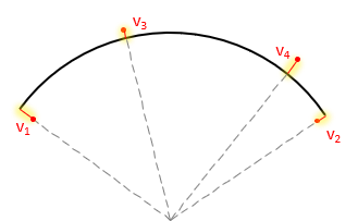
Equations I-10 and I-11 are used to solve the arc if all three points are on the arc, Figure I-13.
| Equation I-10 | |||
 |
Equation I-11 | ||
 |
|||
| Figure I-11 Only arc points |
|||
Four points allows a least squares solution.
Example
Determine the radius for the arc in Figure I-12 using the coordinates of the four arc points in Table I-4.
 |
| Figure I-12 Least Squares Arc Fitting |
| Table I-4 | ||
| Point |
E | N |
| 1 | 117.68 | 806.74 |
| 2 | 690.37 | 795.29 |
| 3 | 316.93 | 940.81 |
| 4 | 618.34 | 873.55 |
Use the coordinates and Equation I-10 to set up the observation equations. Include a residual on the constant term.

Create the initial matrices

Intermediate matrix

Solution matrix

Substitute the solution coefficients into the arc equation.
![]()
Determine the curve radius

Residuals
The observation equation form of equations I-9 and I-10 are:
| |
Equation I-12 |
| |
Equation I-13 |
In Equation I-12 the residual is on the radius which is a function of the coordinates.
In Equation I-13 the residual is on the arc point coordinates.
This makes the residuals perpendicular to the arc (radial), Figure I-13, since there is no dependent-independent variable condition.
 |
| Figure I-13 Curve Fit Residuals |