2. Vertical Curve
Table I-3 lists some elevations at particular stations through which it is desired to run a vertical alignment curve.
| Table I-3 | |
| Station | Elevation |
| 11+00 | 848.8 |
| 12+00 | 850.7 |
| 13+00 | 851.1 |
| 14+00 | 850.3 |
A verical curve is part of a parabola whch is a second-degree polynomial. That means its equation includes a squared independent variable term, Equation I-8.
| y = ax2+bx+c | Equation I-8 |
Where two points are needed to define a straight line, three points are needed for a second-degree polynomial. Why three points? Because there are three unknown coefficients: a, b, and c. More than three allows a least squares solution; each point beyond three is a redundancy.
We don't have to stop there. We can get much more complex: a nth degree polynomial needs n+1 points to fix and >n+1 points for a least squares solution. However, we'll stick to second degree polynomials for now since they cover the bulk of complex survey curves.
The data in Table I-3 is plotted in Figure I-11 along with a best-fit parabolic curve.
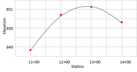 |
| Figure I-11 Best-Fit Vertical Curve |
To determine the curve equation, Equation I-8 is used to develop the observation equations, with the residual term on the Y (Elevation) value.
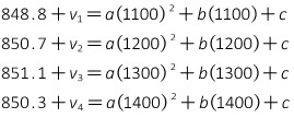
The matrices are:

Now we just solve the matrix algorithm [U] =[Q] x [CTK]
Intermediate products:

Coefficients:

The equation is:
![]()
Notice that many intermediate matrix elements are either extremely large or small. That's not an issue using software to manipulate the matrices, but manual calculations can lead to errors. One way to lessen potential errors is to divide the stations by 100, reducing their size. The observation equations coefficient matrix becomes:

The [Q] matrix:

And the coefficients:

Compare the these coefficients with the solution using the full station expression:
a increases by 10,000 = 1002 which corresponds to a2
b increase by 100 which corresponds to b
c is the same
That means the equation can be written as
![]()
or
![]()
where S = Sta/100